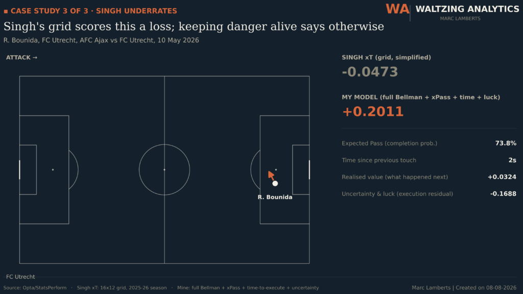
Robert Bounida plays a short pass inside the box. Backwards, almost — five metres, nothing that would make a highlight reel. The traditional way of scoring it, the model that’s run public football analytics since 2018, says this pass lost value: −0.047. A mistake, by the numbers. Something a coach might flag in a debrief.
The model in this article says +0.201. Not a small correction — a flipped sign. One says this pass made the team worse off. The other says it was one of the more valuable actions of the game.
They can’t both be describing the same reality well. This article is about why they disagree, what you have to change to get the second number, and what breaks — computationally, statistically, conceptually — along the way. Two more passes like this one are waiting near the end, once every piece of the model has been built.
What happens when you stop simplifying the Bellman equation, one assumption at a time.
Value models in sport fascinate me. They truly do. How do we assign value to actions on the pitch in relation to scoring goals or preventing goals being scored? That’s the fundamental question that keeps me going every single day. There are some big models that have become household names at this point, like Expected Goals (xG). While xG says more about shot and shot conversion, I want to look at the value on the pitch that creates danger or threat from progression.
There are other value models worth knowing — TransferLab’s goals difference added, American Soccer Analysis’s goals added, StatsBomb’s On-Ball Value, KU Leuven’s VAEP. Links to all of them are in Sources at the end. While each has its own strengths and challenges, none has become as widely used as Expected Threat.
This isn’t really an article about launching a new stat. It’s an investigation into one specific, very well-loved model — what it quietly assumes away to stay simple, and what actually happens, on four real seasons of Eredivisie data, when you put those assumptions back one at a time. The Bounida pass above is the payoff. Everything before it is how you get there.
Contents
- Expected Threat
- Theoretical framework: Markov Decision Process & Bellman Equation
- Data
- Traditional xT
- Create the model without simplification
- Contextual model
- Adding Expected Pass
- Adding Time-to-Execute
- Adding Uncertainty & Luck
- Three Passes, One Model
- Results
- What the model changes in practice
- Netlify App
- Challenges
- Multi-agent reinforcement learning — where this goes next
- Final thoughts
- Sources
1. Expected Threat
This model has had a really big influence on my way of thinking in football. It introduced me to advanced analytics, and showed how a seemingly niche model can become mainstream.
It was introduced by Karun Singh, currently a Research Engineer at Arsenal. You can read the full story in his original post, Introducing Expected Threat (xT).
Soccerment puts the core idea well:
The basic idea behind xT is to divide the pitch into a grid, with each cell assigned a probability of an action initiated there to result in a goal in the next N actions. This approach allows us to value not only parts of the pitch from which scoring directly is more likely, but also those from which an assist is most likely to happen. Actions that move the ball, such as passes and dribbles, can then be valued based solely on their start and end points, by taking the difference in xT between the start and end cell.
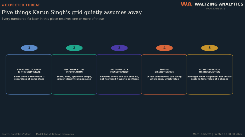
Expected Threat is built from a Markov Decision Process (MDP), and if you know me, I love an MDP in football. It’s genuinely useful for measuring how a player’s dribbles, carries and passes contribute to creating shots. It’s also exactly the model that scored Bounida’s pass as a mistake. Here’s why:
- Starting location is the only state variable. A pass starting in the same zone gets the same value regardless of the game state it was made in.
- There is no contextual information — game state, possession phase, time since ball recovery, tempo of play all go unmeasured.
- No measurement of action difficulty. xT rewards where the ball ends up, not how hard it was to get it there.
- Spatial discretisation, the grid problem. A few centimetres on the pitch can swing which zone — and which value — an action falls into.
- No optimisation or discounting. The model averages what players historically did rather than solving for the best available action, and it treats a chance five actions away as worth exactly the same as a chance right now.
Every numbered section from here on fixes one or more of these five. I’ll call it out explicitly each time so the thread doesn’t get lost — and by Section 10, Bounida’s pass will make sense.
2. Theoretical framework: Markov Decision Process & Bellman Equation
Markov Decision Process
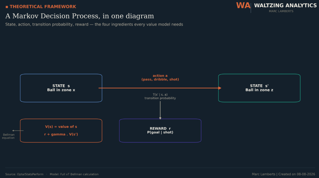
A Markov Decision Process (MDP) is a mathematical framework used to model sequential decision-making in environments where the outcome of an action is uncertain. An MDP is defined by a set of states, a set of possible actions, transition probabilities describing how the system moves between states, and rewards that quantify the benefit of reaching a particular outcome. The objective is to determine the value of each state by considering not only the immediate reward but also the expected rewards that may follow.
The defining assumption is the Markov property: the future depends only on the current state and the action taken, not the complete history that preceded it. In football analytics this suits modelling ball possession well — each action changes the state of the game and shifts the likelihood of future scoring. Expected Threat treats each possession as a series of state transitions, valuing the movement of the ball between areas of the pitch on exactly this principle.
Bellman equation
The Bellman equation is the recursive equation used to determine the value of a state within an MDP. Rather than evaluating an action solely by its immediate outcome, it combines the immediate reward with the expected value of every possible future state that may follow — so the value of a state reflects both its present contribution and its potential to generate future reward.
Within xT models, the Bellman equation estimates the value of possessing the ball in different pitch locations: the probability of scoring directly from a location, combined with the expected value of progressing into more dangerous areas. Repeatedly updating these state values until they converge gives a stable read on how threatening each game state is — the mathematical foundation for valuing passes, carries, and everything else that moves the ball.
3. Data
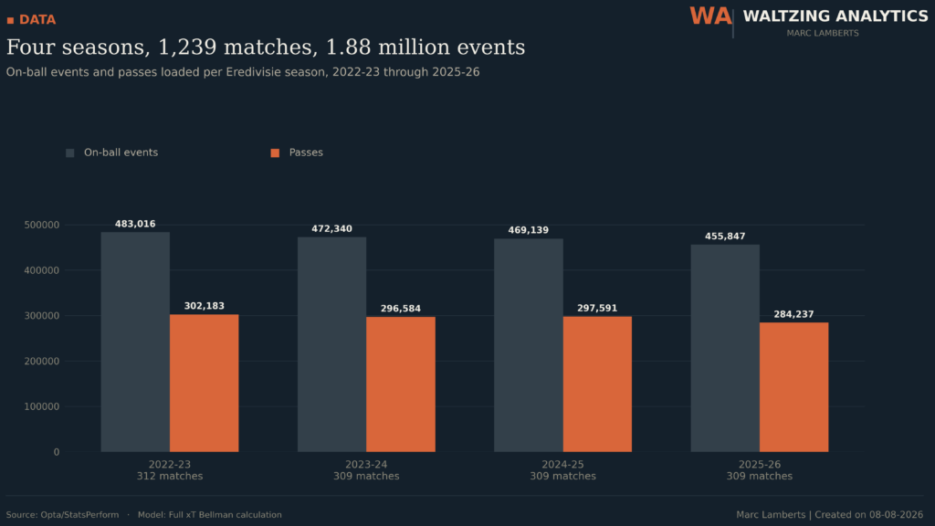
I need enough events to drown out noise, reduce the influence of outliers and luck, and be confident the model has actually seen enough football to generalise. I collected four full seasons of Eredivisie data via the Opta/StatsPerform API — 2022–23 through 2025–26 — data pulled on 2 August 2026.
Across the matches I was able to load and process: 1,239 matches, 1,880,342 on-ball events, of which 1,180,595 are passes. That figure includes play-off games for Europe and against relegation. (My internal count landed a few matches under the 1,244 in my original collection notes — a handful of files weren’t present in the load folder at processing time. Worth reconciling against the raw archive before publishing a final number.)
4. Traditional xT
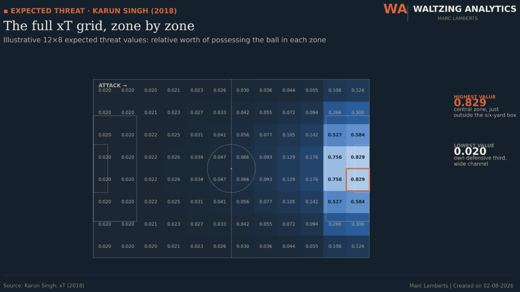
As covered above, Karun Singh’s Expected Threat is the traditional starting point. To build something new, you have to understand what exists.
The pitch is divided into a grid, and every bin carries a value. xT for an action is the difference between the value of the ending bin and the value of the starting bin — that’s the entire scoring mechanism. It’s also, mechanically, exactly what produced Bounida’s −0.047: his pass moved the ball from a slightly-better-looking bin to a slightly-worse-looking one, and the grid has no way to know anything else about the moment.
Two patterns fall out of the grid immediately. First, passing is the dominant progression action almost everywhere on the pitch — it’s only once you’re inside the box that shooting starts to rival it in value terms. Second, average xT added is highest on long passes, then medium, then very long, then short — length alone is doing real work. And when you rank the highest-value origin zones specifically, they cluster entirely in the attacking third, with the central attacking channel well ahead of everything else.
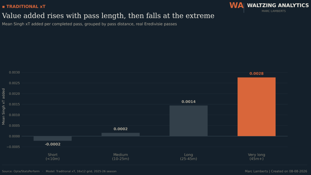
This model has been used worldwide since 2018. What’s less well known is exactly how simplified a version of the Bellman equation it actually is.
5. Create the model without simplification
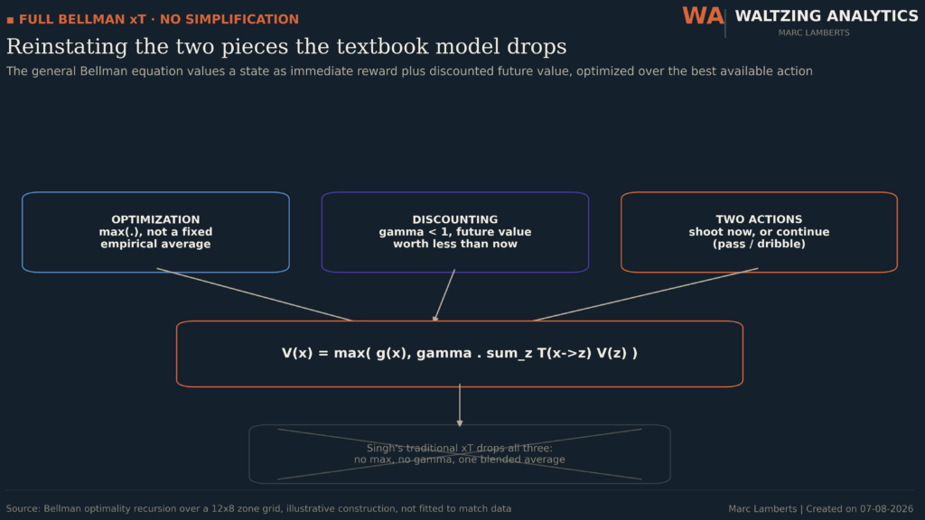
Start with what Singh’s xT actually computes:
V(x) = s(x)·g(x) + (1 − s(x))·Σ T(x→z)·V(z)
That’s a weighted average of “shoot now” and “keep the ball,” blended by how often players historically chose each option — not by which one was actually better. There’s no discount factor either, so a chance five passes away counts exactly as much as a chance right now. (This is problem #5 from Section 1.)
Karun Singh took the general Bellman equation and stripped it to the minimum needed for a purely spatial model. He collapsed the state to nothing but the ball’s pitch zone — problem #1. He dropped every piece of context: score, time, opponent shape, player identity — problem #2. He collapsed the action space to two outcomes, shoot or move, with probabilities taken from historical frequency rather than optimised — there’s no max operator anywhere, just an expectation over a fixed, empirically observed policy. The transition probabilities for the move branch come from one league-wide matrix, averaged over every player and situation rather than conditioned on the specific one in front of you. Reward is reduced to a single sparse term — probability of scoring given a shot — so a turnover isn’t modelled as a real event with a real state; it simply isn’t part of the “successful move” mass. And there’s no discount factor at all: convergence comes for free because some shot probability always exists in every zone, so value stops accumulating after a handful of iterations regardless.
The real Bellman equation doesn’t blend — it optimises:
V(x) = max( g(x), γ · Σ T(x→z)·V(z) )
Two changes: a max operator (take the better of shoot-now vs. continue, don’t average them) and a discount factor γ (future value is worth less than present value). Put them back and you get an optimal stopping problem — the same mathematical structure as deciding when to sell a stock, not a Markov chain you passively evaluate.
Solved on the same synthetic 12×8 grid as a like-for-like comparison, the shape changes in a specific way: the simplified model blends smoothly from midfield into the box, because it’s always averaging. The optimised model creates a hard edge — the exact zone where shooting becomes strictly better than continuing — because max() doesn’t blend, it picks.
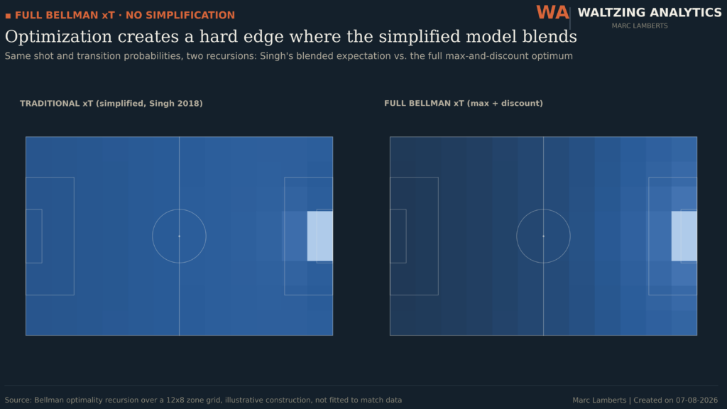
This version is illustrative, not fitted — the point was isolating exactly what optimisation and discounting change before adding anything else. Every section from here on runs on real data.
6. Contextual model
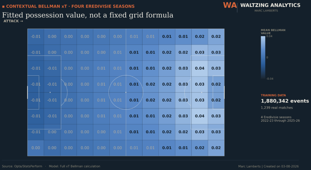
Grid-based xT has a ceiling: it can only ever know which of 96 zones the ball is in. It has no idea if a defender is goal-side, whether the team is protecting a lead, or how the last three touches went. Fixing that means giving up the closed-form equation entirely and fitting the value function instead — which is how this section resolves problems #1, #2, and #4 from Section 1 all at once: state stops being “which of 96 boxes,” context becomes an explicit input, and the pitch coordinates the model trains on are continuous, never binned. The grid only comes back later, for display.
The approach, adapted from a reference notebook built for exactly this: two gradient-boosted classifiers predict P(team scores in the next 10 actions) and P(team concedes in the next 10 actions) from roughly 30 continuous features per event — coordinates, action type, possession phase, score state, time elapsed. State value is the difference of the two. A regressor then repeatedly re-fits the Bellman target y = reward + γ·V(next_state) across several iterations — fitted value iteration, where each round of “solving” the equation means training a new model, not evaluating a formula.
Run end-to-end on all four seasons — 1.88 million events, GroupKFold split by match so no match ever leaks between train and validation — the full pipeline finishes in under 15 minutes.
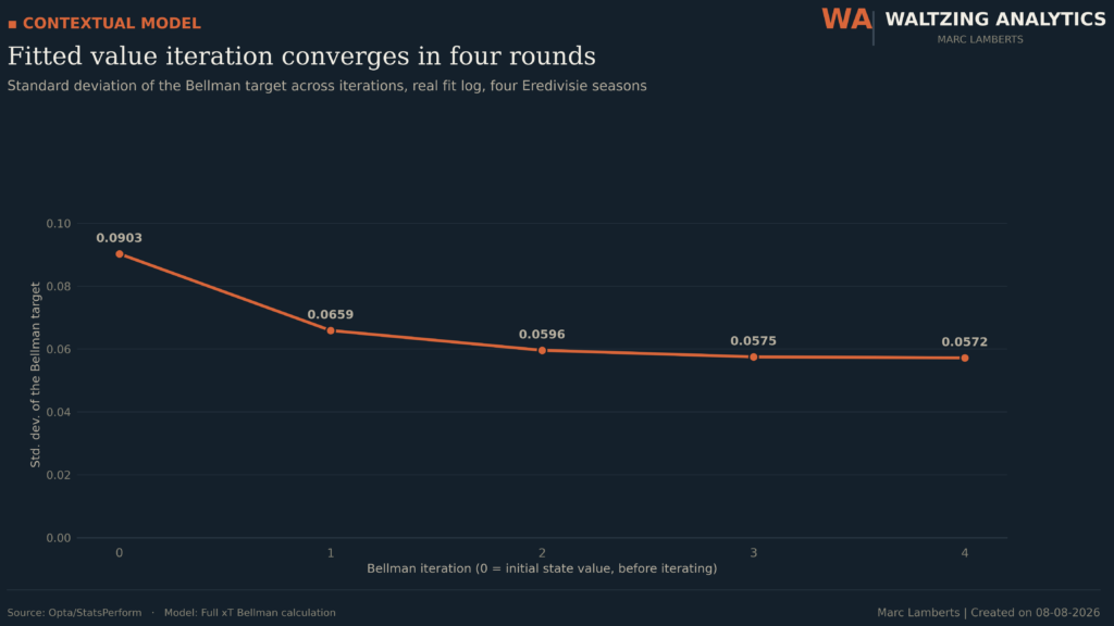
From here I’ll call this fitted, context-aware value function CxT — Contextual Expected Threat. Every result for the rest of this article is CxT, not Singh’s original formula. This alone already changes Bounida’s number, but not the whole way — two more pieces are still missing.
7. Adding Expected Pass
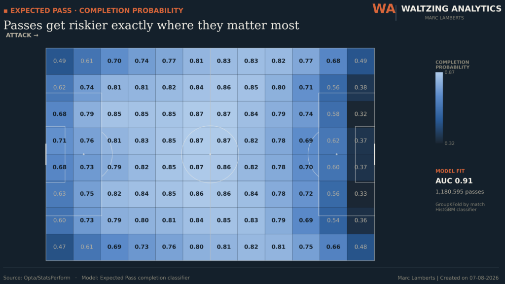
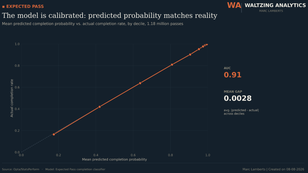
Every version so far assumes a pass reaches its target. It doesn’t — completion rate across four Eredivisie seasons is 78.4%, and it isn’t uniform. This is problem #3 from Section 1, tackled directly: a separate classifier, fit only on the 1,180,595 real pass events (distance, angle, pressure proxies, score state), predicts completion probability directly — AUC 0.91, calibrated to within 0.001 of the true rate.
The pattern runs exactly backwards from what you’d want if you were only optimising for safety: completion probability is highest in central midfield (0.85–0.87) and falls off a cliff toward the byline and the corners of the box, down to 0.32–0.49. The zones that matter most for value are the zones least likely to actually connect — so any value model that doesn’t weight by completion probability is systematically overrating risky final-third passing.
8. Adding Time-to-Execute
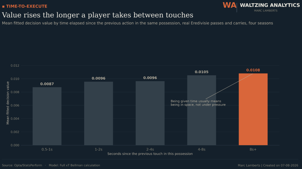
The Bellman equation discounts by step, not by time — a second half of problem #3, and a piece of problem #2 as well. Five actions in three seconds and five actions in thirty seconds get discounted identically, which is obviously wrong: a chance three seconds away is worth more than the same chance thirty seconds away, but “step count” can’t tell the difference.
Using the real gap between touches (seconds_since_prev, already logged for every event) grouped into buckets, the result runs opposite to the “quick combination play is more valuable” intuition: value rises the longer a player takes, from 0.0087 under one second to 0.0108 past eight seconds. The likely reason isn’t that slowness helps — it’s confounding by what slowness means. Being given time on the ball usually means being unmarked, in space, not under pressure, and those are exactly the situations that carry higher value regardless of tempo. A cleaner version of this feature would need to separate “time because nobody’s closing you down” from “time because you’re static and the move has stalled,” which per-touch gap alone can’t do. Flagging it, not fixing it here.
9. Adding Uncertainty & Luck
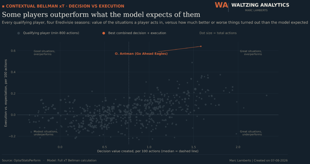
None of the fixes so far touch a limitation Singh’s model has by construction, not by simplification: a model that only outputs “expected value” can’t tell you whether a player is actually good or just fortunate. This is the one genuinely new capability in this article rather than a repair of one of the original five problems — and it’s the piece that turns Bounida’s pass from “a different number” into “a different story.”
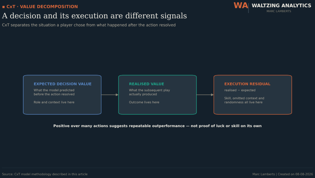
The decomposition, adapted from the same reference notebook, solves this cleanly: expected_decision_value is what the model predicted before the action resolved; realised_value is what actually happened next; execution_residual is the gap between them. Positive residual, sustained over hundreds of actions, means a player is outperforming what the situations they’re in would predict — the closest thing this framework has to isolating skill from context.
O. Antman (Go Ahead Eagles) leads the combined measure — not because he’s involved in the highest-value situations (Tadić and Bergwijn create more valuable positions on paper) but because he outperforms what his situations predict by the widest margin. That’s a genuinely different signal than “creates a lot of CxT,” and it’s only visible once expectation is decomposed from outcome. PSV Eindhoven players take 6 of the top 9 overperformer spots.
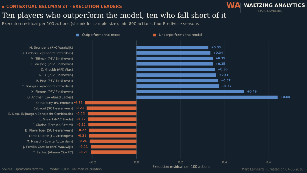
Worth being honest about: none of this is really “luck” in the strict sense. It’s whatever the model’s features didn’t capture, which includes real skill, finishing quality, and yes, some randomness. The honest name for the residual is “unexplained,” and luck is only one component of that.
Every piece is on the table now. Time to go back to the pitch.
10. Three Passes, One Model
Three real, completed passes from the 2025–26 season, each valued twice: once by Singh’s static grid, once by the full stack built across Sections 5 through 9 — optimisation and discounting, contextual fitting, Expected Pass, and the execution/luck decomposition, all at once.
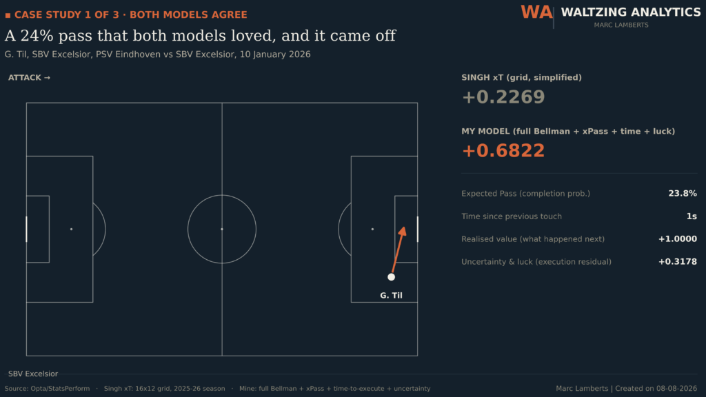
G. Til’s pass into the six-yard box is where both models agree, at least in direction — Singh scores it +0.227, CxT scores it +0.682. What Singh can’t show you is why the gap is that wide: this was a 23.8% pass by completion probability, and it worked, for a +0.318 execution residual. Both models liked the decision. Only one of them tells you it was a coin-flip that came off.
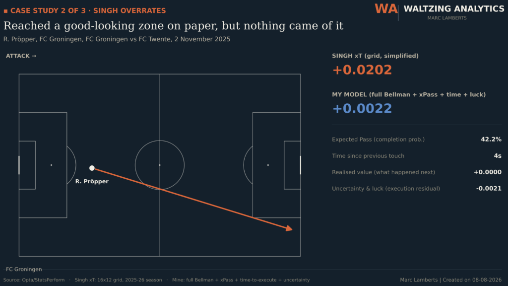
R. Pröpper’s long diagonal switch reaches a zone Singh’s grid rates well — +0.020, comfortably top 2% of all passes that season. CxT rates it at +0.002, next to nothing. The completion odds were only 42%, and — because the pass is scored on realised value, not just on reaching the zone — the actual continuation amounted to nothing: 0.000024, functionally zero. Reaching a good-looking zone and something coming of it are different events. Singh’s grid can only ever measure the first one.
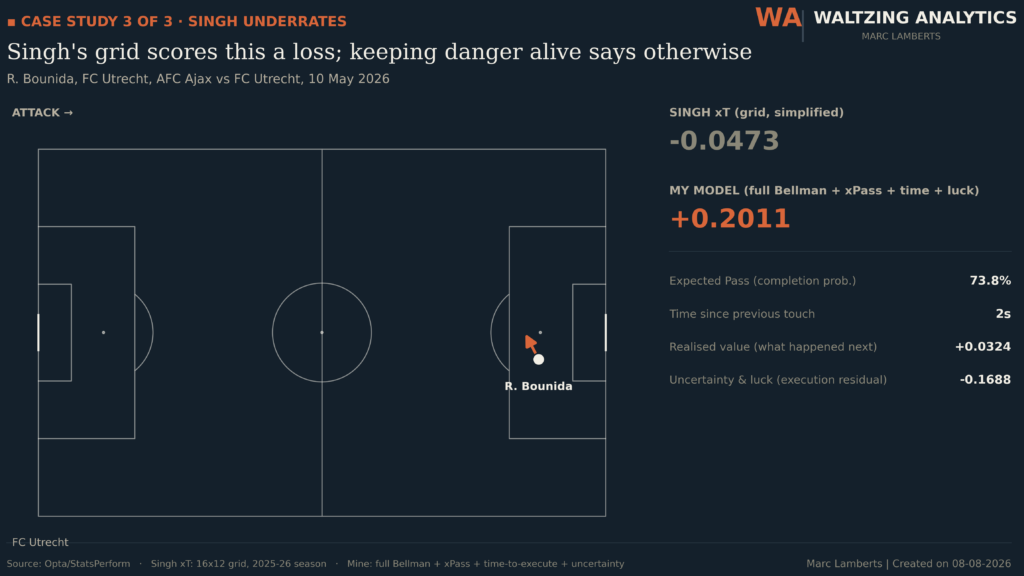
And Bounida’s pass, from the top of this article. Singh: −0.047, a value loss, purely because the end zone scores marginally lower than the start zone on the static grid. CxT: +0.201. The completion odds were high, 73.8%, and the context — a short ball that keeps the move alive inside the box rather than resetting it — is worth something Singh’s zone-delta structurally cannot register, because zone-delta has no concept of “the move stays alive.” The execution residual is negative, −0.169, meaning even CxT’s own optimistic pre-pass expectation didn’t fully pay off. But it never went negative. Singh’s model was never in a position to know that; it scored the pass as a mistake before the move even continued.
Three passes. Three different reasons the numbers disagree — a probability the simple model can’t see, a continuation the simple model doesn’t check, and a context the simple model has no state variable for. That’s the whole article, in three arrows on a pitch.
11. Results
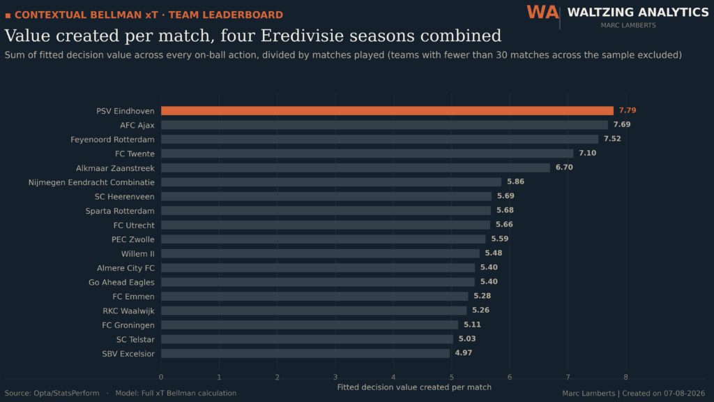
Pulling the fitted model across all four seasons together, a few aggregate patterns hold up before getting into individual cases:
Teams. Ranked by fitted decision value created per match, the leaderboard reads the way you’d expect a competent model to read: PSV Eindhoven, AFC Ajax, Feyenoord Rotterdam and FC Twente occupy the top of the table. That’s a useful sanity check in itself — a model that put a mid-table side above PSV would be a model to distrust, not admire.
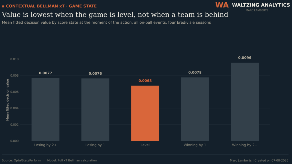
Game state. Value is lowest when games are level (0.0068) and highest when a team is up by two or more (0.0096) — tight, contested games produce the least valuable actions on average, not the most desperate ones.
Execution leaders. The top and bottom 10 players by execution residual single out players over- and under-performing their situations specifically, separate from who’s simply involved in the most dangerous moments.
Top passers and carriers. D. Tadić leads passing value per 100 passes at 2.81, on the largest sample in the top 10 (1,224 passes) — not a small-sample fluke. S. Lammers tops the carrying table at 4.12 per 100 carries, though on only 36 attempts — read that one as “who to watch,” since carries are rare enough (45,809 total, against 1.18 million passes) that the qualifying threshold still leaves the top of the table noisy.
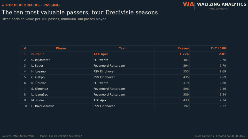
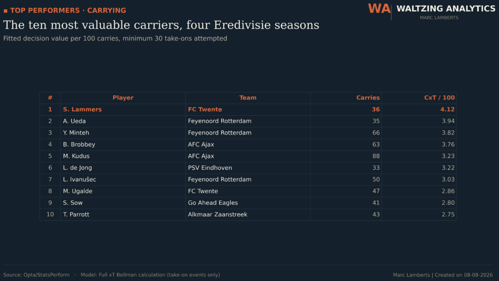
(One methodological note worth including, because it nearly went into this article wrong: an earlier “net action value” metric — a raw Bellman temporal-difference term — ranked PSV dead last on the team leaderboard, directly contradicted by the same team sweeping the execution leaderboard. The metric doesn’t track team quality; it conflates real value creation with the ordinary decay of sitting in an already-good position. Checking correlations against a metric everyone agrees behaves sensibly, expected_decision_value, before trusting a leaderboard is what caught it.)
12. What the model changes in practice
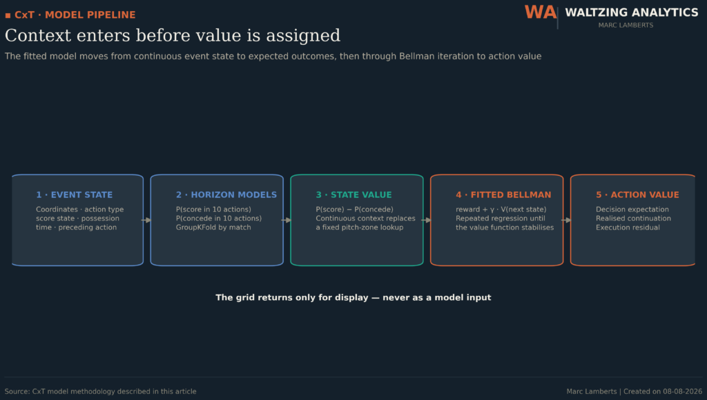
The most useful change is not a prettier pitch map. It is a different answer to a football question. Traditional xT asks: did the ball move into a more valuable zone? CxT asks: given the situation, the difficulty of the action and what followed, how much did this decision change the team’s prospects?
That distinction changes what a leaderboard means. A player can create valuable situations because of role and territory, execute difficult actions better than expected, or do both. CxT keeps those ideas separate. It also makes failure informative: an ambitious pass that does not connect can still be a defensible decision, while a completed pass into an attractive zone can contribute almost nothing if the possession immediately dies.
The three passes above are therefore more than examples. They are three tests of whether the model sees the game we think we are measuring: risk, continuation and context. The aggregate results suggest it does, but they should be treated as validation evidence rather than proof. The real test is whether these signals remain stable across seasons, competitions and unseen matches—and whether coaches and analysts recognise the decisions the model rewards.
14. Challenges
A few things that actually went wrong or slowed things down while building this, worth naming rather than glossing over:
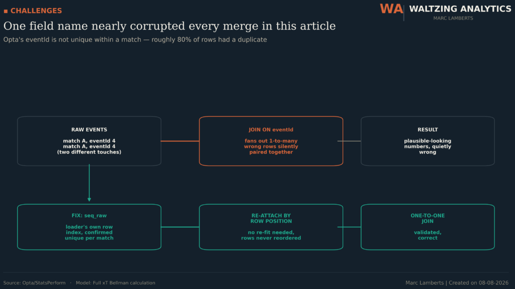
The event_id field is not a safe join key. Opta’s eventId is not unique within a match — roughly 80% of rows in the full dataset had duplicate (match_id, event_id) pairs. Every merge using that key silently fanned out into incorrect many-to-many joins. The fix was switching to the loader’s own row-enumeration index, confirmed unique, and re-attaching it by row position rather than re-running the affected pipeline stages from scratch. This is the kind of bug that doesn’t crash anything — it just quietly produces plausible-looking wrong numbers, which is worse.
Not every metric that looks like “value created” is. A raw Bellman temporal-difference term (net_action_value) was the first thing tried for the team leaderboard. It ranked PSV dead last. That’s not a research finding, it’s a metric that conflates genuine value creation with the ordinary mathematical decay of sitting in an already-good position — see the note under Results.
Small samples are everywhere once you split by action type. Carries are rare enough — 45,809 against 1.18 million passes — that per-player carrying leaderboards need real sample-size discipline (minimum action counts, shrinkage toward zero) or the top of the table is just noise wearing a ranking.
Time-to-execute has an unresolved confound. Covered honestly in Section 8: the feature can’t currently distinguish “given time because there’s no pressure” from “stalled because the move broke down.” Both look identical as a single number of seconds.
Runtime is real, even with efficient tooling. Fitting on 1.88 million events with GroupKFold cross-validation and gradient boosting takes on the order of 10–15 minutes end-to-end. Not slow by research standards, but slow enough that iterating on feature choices costs real time, not instant feedback.
15. Multi-agent reinforcement learning — where this goes next
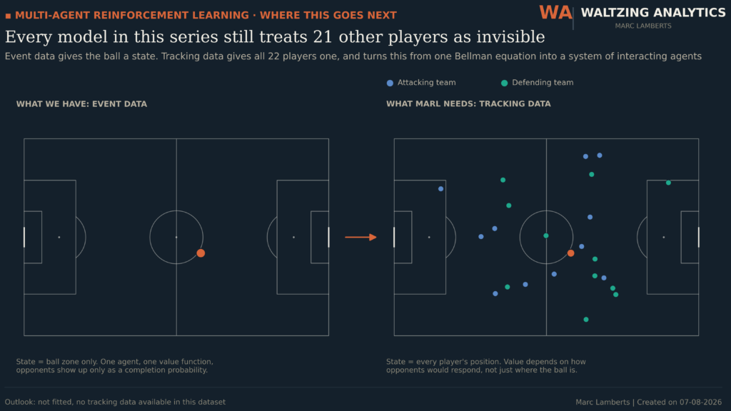
Every model in this article, however sophisticated the fitting, still describes one agent — the ball — moving through a world where the other 21 players are compressed into a single number: a completion probability, a shot probability. Real football isn’t single-agent. It’s 22 people simultaneously updating their positions in response to each other, and the value of a pass genuinely depends on how defenders would respond to it, not just a historical average of how they usually have.
Getting there needs tracking data, not event data — full player-position streams, not just touches. With it, the framing shifts from one Bellman equation to a system of interacting agents: multi-agent reinforcement learning, where attacking players and defending players are separately-optimising agents in the same environment, and equilibrium concepts — not just expectation — start to matter. That’s a genuinely different research program, not a tweak to this one, which is exactly why it’s the outlook section and not a fitted result. Nothing in this article claims otherwise.
16. Final thoughts
Start over, one more time, from the top: a pass that a beloved, decade-old model scores as a mistake, and isn’t. That’s not a gotcha aimed at Karun Singh — the grid he built was never trying to be a full MDP, it was trying to be usable with nothing but event data and an afternoon, and it succeeded so completely that it’s still the default eight years later. The gap between −0.047 and +0.201 isn’t a bug in his model. It’s the sum of every simplification he made on purpose, all landing on one five-metre pass at once.
The single biggest jump in closing that gap wasn’t any individual fix in Sections 7 through 9. It was Section 6 — the decision to give up the closed-form grid entirely and let a model fit the value function from continuous context instead of reading it off 96 boxes. Everything after that — pass risk, urgency, the gap between what a player was expected to do and what actually happened — is pricing in what the grid version was structurally never going to see, no matter how it was tuned.
The honest caveats matter as much as the results. This is one league, four seasons, event data rather than tracking data, and — until Section 15 becomes a fitted result instead of an outlook — still fundamentally a single-agent model wearing a 22-player sport’s clothing. None of that makes CxT wrong. It makes it a specific, well-understood set of trade-offs, which is a better place to stand than a model whose simplifications nobody wrote down — including, until now, the one that gave a five-metre pass a minus sign.
17. Sources
- Karun Singh, Introducing Expected Threat (xT)
- TransferLab, Goals Difference Added
- American Soccer Analysis, What Are Goals Added?
- StatsBomb, Introducing On-Ball Value (OBV)
- KU Leuven DTAI Sports Analytics Lab, VAEP
- All data: Opta/StatsPerform event feeds, Eredivisie 2022–23 through 2025–26, collected 2 August 2026.
- All models: HistGradientBoosting classifiers/regressors, GroupKFold cross-validated by match.