
You know what I have underestimated for years? Communication in football. Whether that is within a football organisation, on social media or talking to your peers. The key to all your ideas is communication, more specifically, language. If you speak the same football language throughout all disciplines of the sporting entity, there is a smaller margin for error.
In that spirit, there is also the case where two different words/definitions are loosely thrown around as if they were the same thing. And that is what I want to talk about today. The difference between an outlier and an anomaly.
Contents
- Data
- Theory I: Outlier
- Theory II: Anomaly
- differences
- Scouting I: Outliers
- Scouting II: Anomalies
- Final thoughts
Data
The data I use for this aggregated data. This data consists of my own metrics for the J2/J3 2026 season which have been built on the raw event data of Opta. By creating my own metrics, I have more freedom of what I would like to see, but there is always a chance of error. This data was created on August, 15th, 2026.
I will look at players thave played over 450 minutes and are central forwards/striker as a position. Furthermore, I have created a profile that states that they need to be in the box over 60% of their touches and 80% of their shots should come from that area. This I have done with the raw event data.
Theory I: Outlier
Outliers are data points that significantly deviate from most of the dataset, such that they are considerably distant from the central cluster of values. They can be caused by data variability, errors during experimentation, or simply uncommon phenomena which occur naturally within a set of data. Statistical measures based on interquartile range (IQR) or deviations from the mean i.e. standard deviation, are used to identify outliers.
In a dataset, an outlier is defined as one lying outside 1.5 times the IQR from either the first or third quartile, or 3 standard deviations from the mean. These extreme figures may distort analysis and produce false statistical conclusions, thereby affecting the accuracy of machine learning models.
Outliers require careful treatment since they can indicate important anomalies worth further investigation or simply result from collecting incorrect data. Depending on context, these can be eliminated, altered, or algorithmically handled using certain techniques to minimise their effects. In sum, outliers form part of the crucial components used in data analysis, requiring accurate identification and proper handling to make sure results obtained are strong and dependable.
Homogeneous and heterogeneous outliers
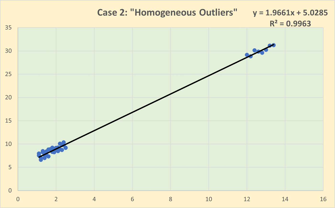
Homogeneous outliers are data points that deviate from the overall dataset but still resemble each other. They form a group with similar characteristics, indicating that they might represent a consistent pattern or trend that is distinct from the main data cluster. For example, in a dataset of human heights, a cluster of very tall basketball players would be homogeneous outliers. These outliers might suggest a subgroup within the data that follows a different distribution but is internally consistent.
Press enter or click to view image in full size
Credit: Winning with Analytics, 2023
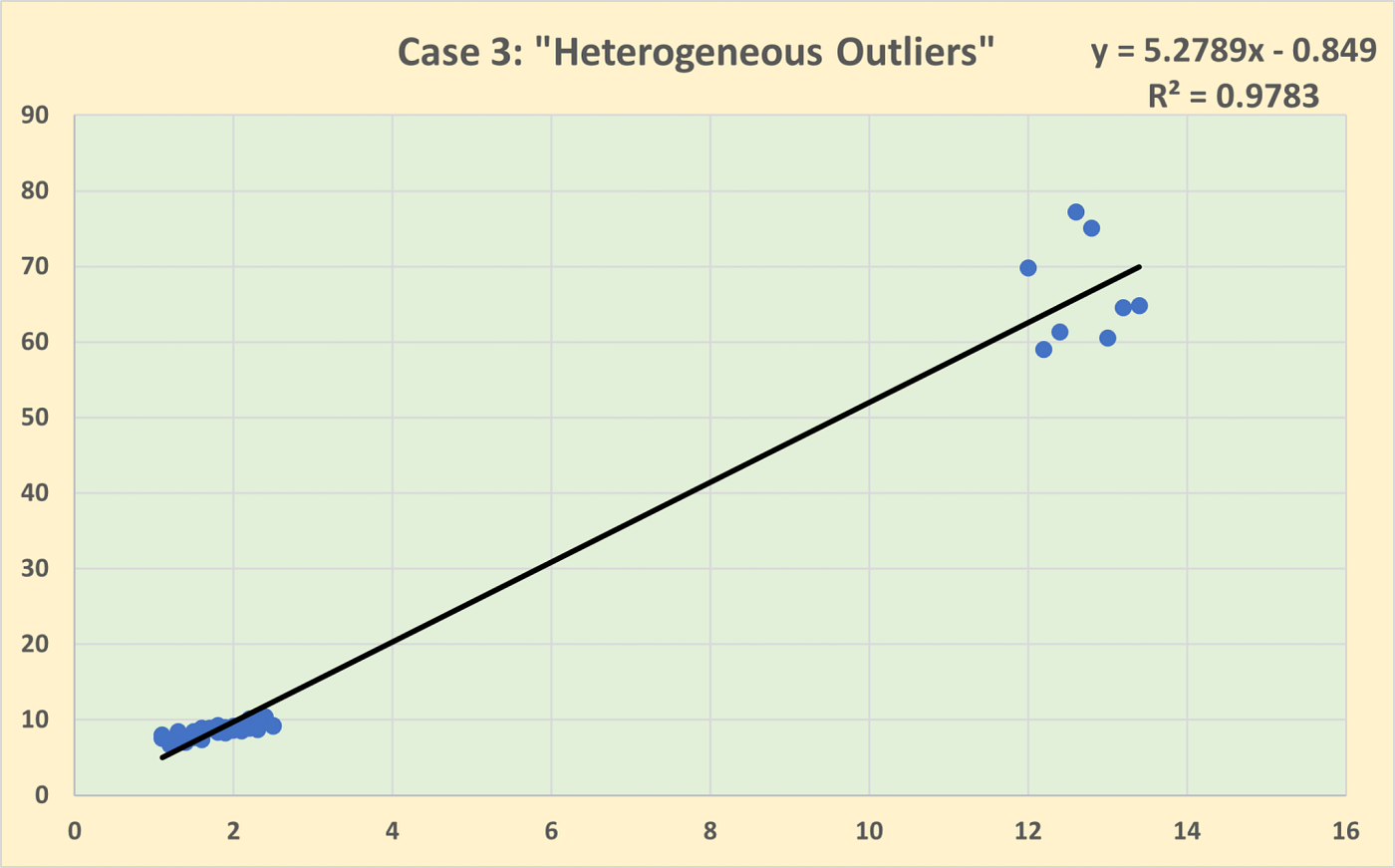
Heterogeneous outliers, on the other hand, are individual data points that stand out on their own, without any apparent pattern or similarity to other outliers. Each heterogeneous outlier is unique in its deviation from the dataset. Using the same height example, a single very tall individual in a general population dataset would be a heterogeneous outlier. These outliers might be due to data entry errors, measurement anomalies, or rare events.
Credit: Winning with Analytics, 2023
Theory II: Anomalies
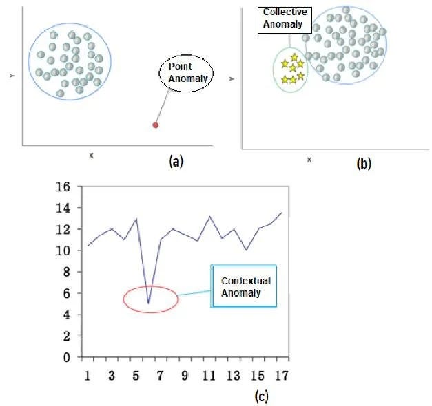
Anomalies are observations, patterns, or behaviours within a dataset that differ significantly from what would normally be expected. They represent unusual occurrences that do not follow the general structure or behaviour present in the majority of the data. Anomalies can arise because of measurement errors, unexpected circumstances, changes in underlying processes, or naturally occurring rare events. Their presence can therefore provide important information about the behaviour and structure of a dataset.
Local Anomalies
Local anomalies are observations that behave unusually compared with a specific group of similar observations, rather than compared with the entire dataset. They are identified by defining a local neighbourhood around each observation and determining whether its characteristics differ substantially from those of nearby or comparable observations.
Contextual Anomalies
Contextual anomalies are observations that become unusual because of the specific circumstances in which they occur. Their anomalous nature cannot be determined from the observed value alone, because the same value may be expected in one context and unexpected in another.
Contextual anomaly detection therefore separates the context of an observation from its behaviour. Context can consist of variables such as time, location, category, role, environment, or situation. The expected behaviour is first established within that particular context, after which the actual observation is compared with this expectation. The greater the deviation from what is normally expected under those circumstances, the stronger the indication of an anomaly.
Multivariate Anomalies
Multivariate anomalies occur when an unusual pattern emerges from the combination of multiple variables. Individual variables do not necessarily contain unusual values. Instead, it is their particular relationship or combination that makes the observation anomalous.
Conditional Anomalies
Conditional anomalies are observations whose behaviour is unusual given a particular set of known conditions. Their identification is based on estimating what should reasonably be expected after accounting for variables that influence the outcome.
Differences
An outlier is an observation that is statistically distant from the majority of values in a dataset. It is usually identified according to the distribution of a variable, using methods such as the interquartile range (IQR), standard deviations, or z-scores. The main consideration is therefore statistical extremity: an observation is considered an outlier because its numerical value lies unusually far from the central concentration of the data. Outlier detection is consequently often based on relatively clear statistical thresholds.
An anomaly, by contrast, is an observation or pattern that behaves differently from what would normally be expected. An anomalous observation does not necessarily contain an extreme numerical value. Its unusual nature can instead originate from its context, its relationship with other variables, its local environment, or the combination of characteristics it possesses. Anomaly detection therefore focuses on identifying unexpected behaviour or patterns and often uses statistical models or machine learning techniques to establish what constitutes normal behaviour before measuring deviations from it.
The fundamental difference is therefore that outliers concern statistical distance, whereas anomalies concern unexpected behaviour. An extreme value can be perfectly explainable and therefore provide little unusual information, while an apparently ordinary value can become anomalous once its context or relationship with other variables is considered. Outlier analysis primarily asks “How extreme is this observation?”, whereas anomaly detection asks “How unusual is this observation given what we would normally expect?”
Scouting I: Outliers
As said, I’m looking for strikers that have played 900+ minutes, have 60% of their touches in the box, and 80% of their shots in that same region. First, I will show you the distribution plot to show how many players come in that region.
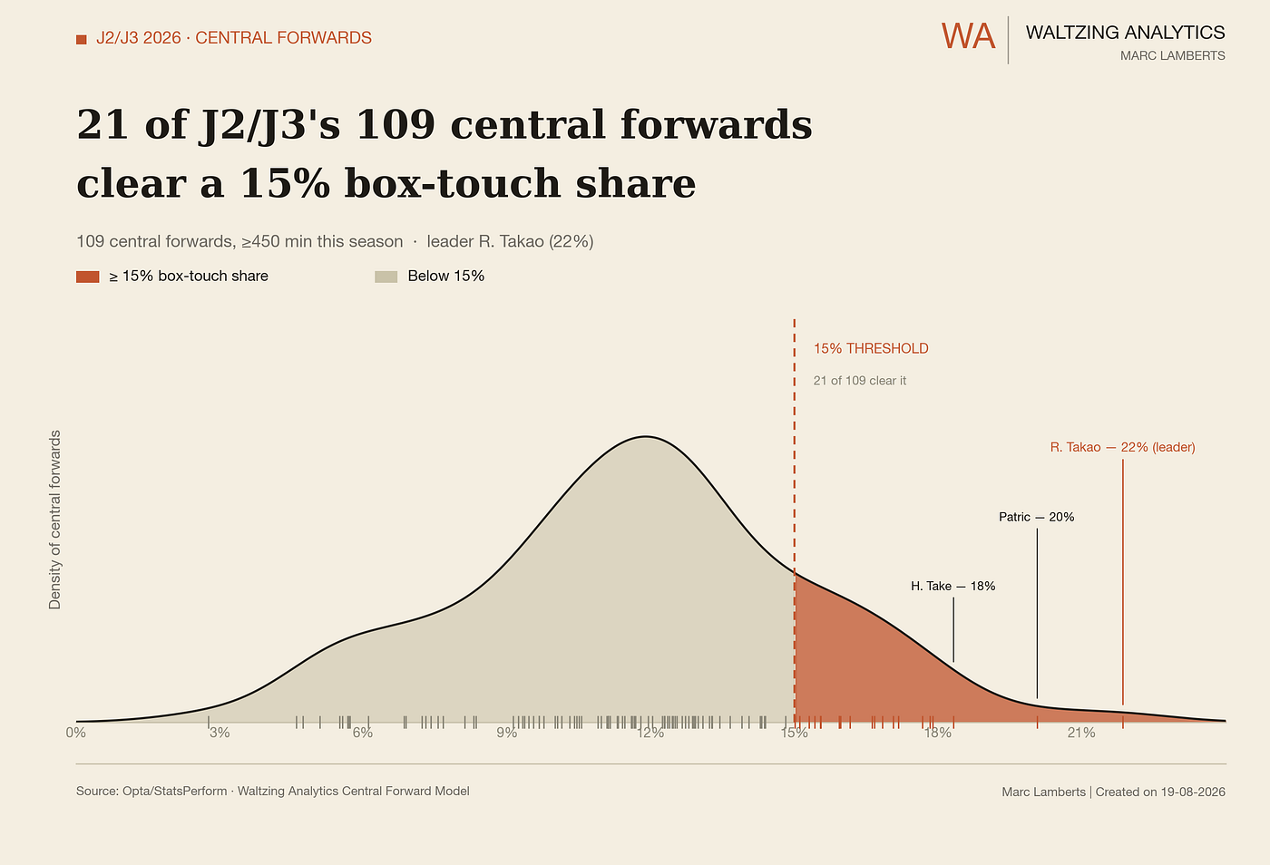
Now I had to rectify something first. There were no players with 60% of their touches in the box. Far from it. I have changed the threshold to 15%, and that left me with 21 players that met that threshold.
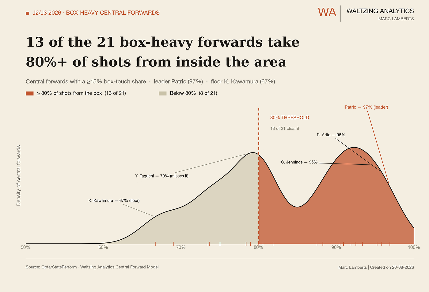
Continuing on those 21 players, we look forward and see that there are 13 players that meet the threshold of 80% of their shots coming from within that specific area. I started the X-axis at 50% because there were no players who scored lower than 60%. That’s for visual clarity.
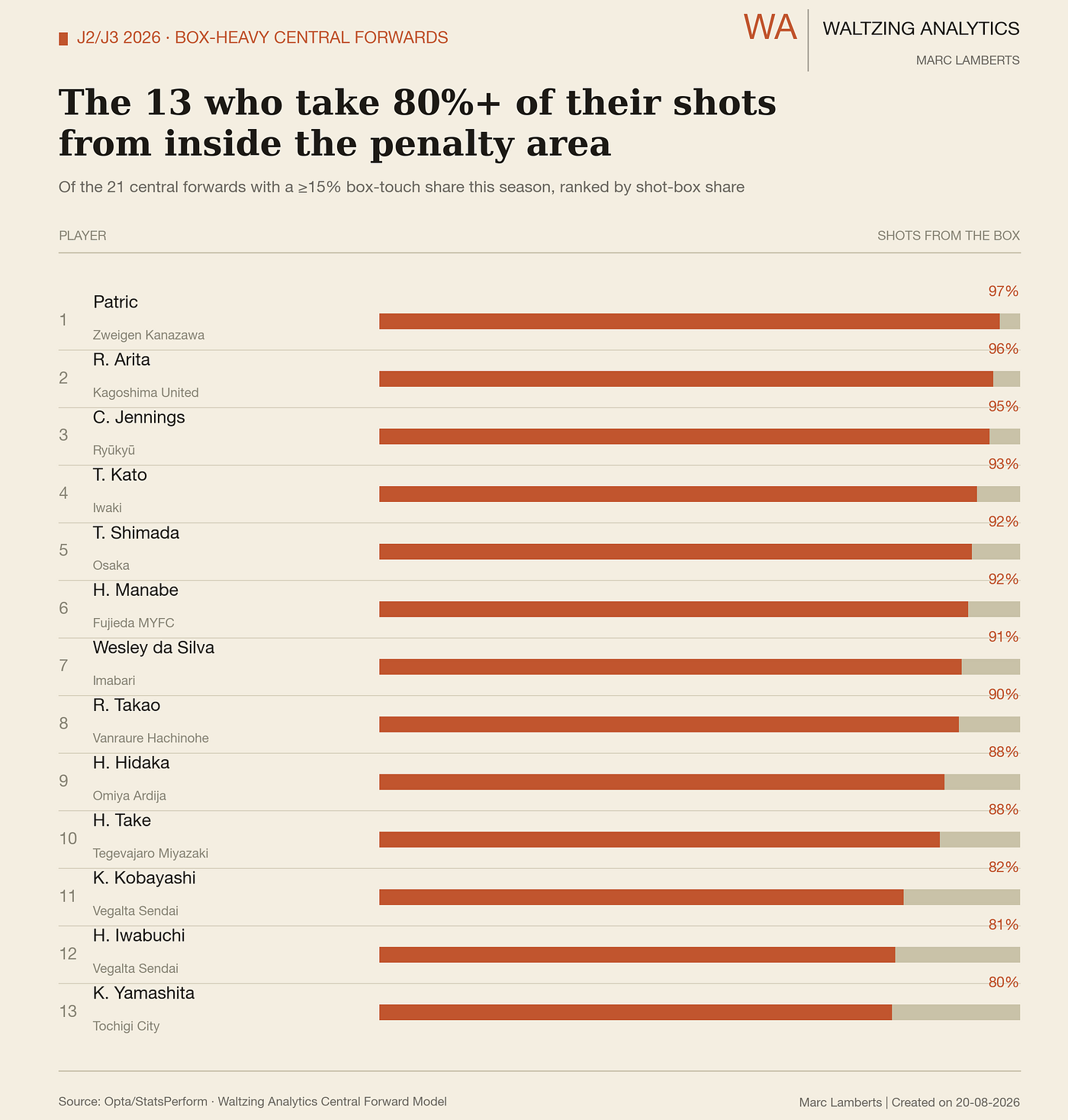
Now I have my players; I want to compare two specific metrics: shots per 90 minutes vs shot conversion %. This will allow me to show how shots compare to the conversion for our selected players who are considered real box threats.
Let’s have a look at the outliers:
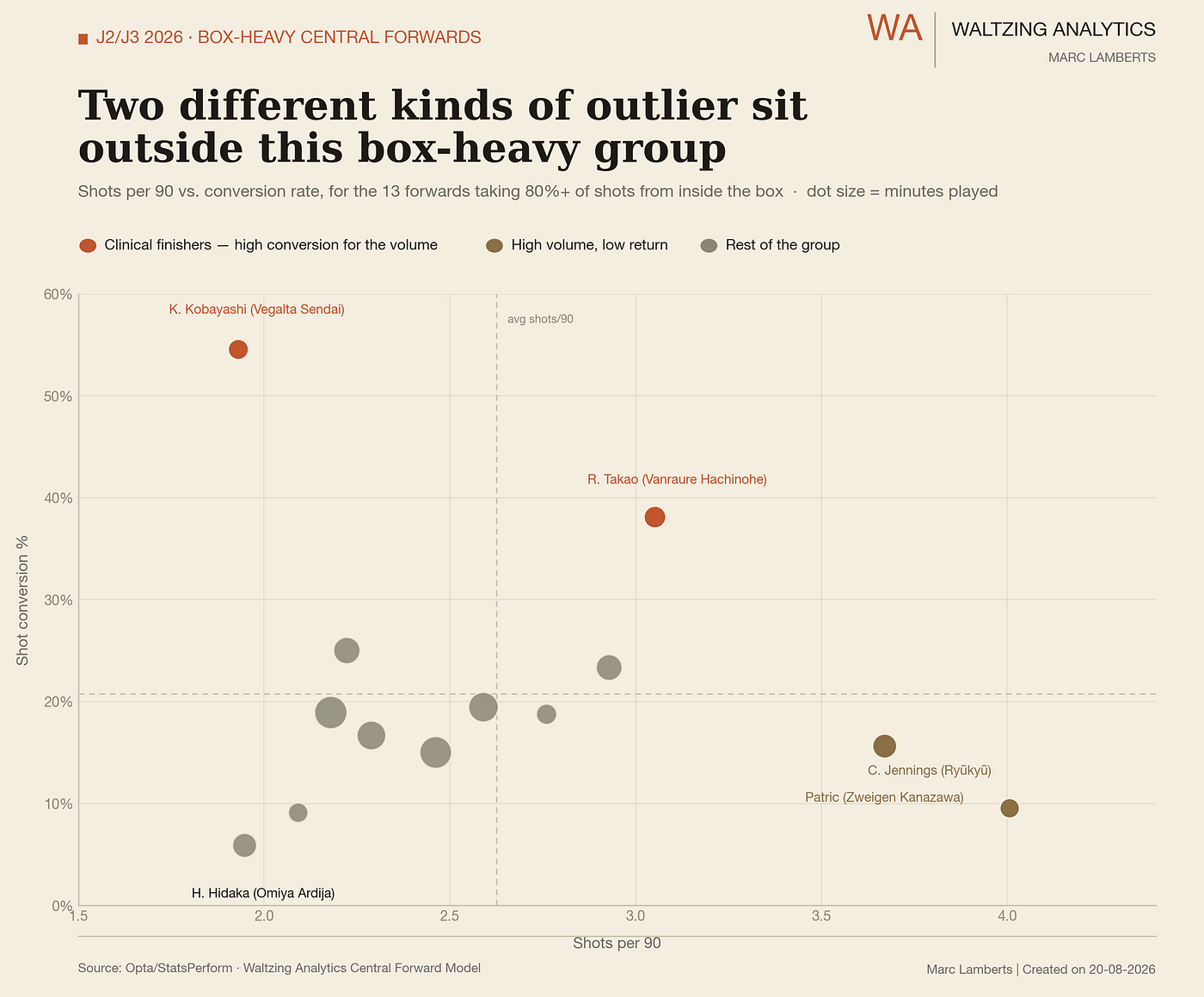
In this scatterplot, we see the two metrics compared. The outliers have gotten a different colour. This is what we call heterogeneous outliers. They are outliers for each particular metric. Jennings and Patric are best in shots per 90, and Kobayashi and Rakao are best in shot conversion %.
Both axes are converted to z-scores (standard deviations from the group average) using the 13 players:
zx= how far a player’s shots-per-90 is from the group average, in standard deviationszy= how far a player’s conversion % is from the group average, in standard deviations
Then two separate, direction-specific rules decide the colour:
- Clinical finisher (coral):
zy > 1.2— conversion rate alone is unusually high, regardless of how many shots they take. Catches Kobayashi and Takao. - High volume, low return (rust):
zx > 1.2ANDzy < 0— shoots far more than average and converts below average. Catches Jennings and Patric. - Anyone not caught by either rule stays gray (“core”).
So, what if we choose to not look at our specifc box, profile and let that go, how would it look like then?
Moving to the next scatterplot:
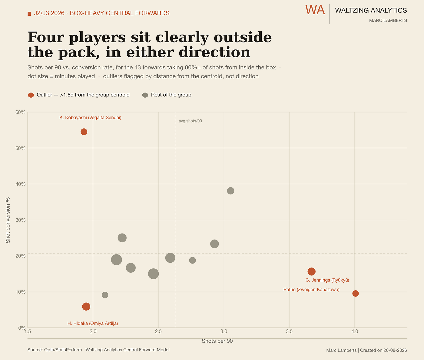
In the scatterplot above, you see the same players against the same metrics. The outliers, however, are not calculated as heterogeneous, but as homogeneous. They are calculated as if they are all composed of one data metric, not mixed. This means that outliers are slightly different.
The outliers here are Kobayashi, Hidaka, Jenning and Patric. Hidaka is a new outlier, while Takao isn’t an outlier according to this metric.
Same two z-scores (zx, zy), but instead of checking direction, they’re combined into a single number — the straight-line distance from the centre of the group:
z_combined = √(zx² + zy²)
If z_combined > 1.5, the player is coloured as an outlier; otherwise, they’re grey. This treats “outlier” as one uniform bucket — it only answers how far out a player is, never which way. That’s why it’s homogeneous: every flagged player gets the same color even though Kobayashi (extreme conversion) and Jennings (extreme volume) are outliers for opposite reasons.
However, I’m not satisfied. These filters are too strict. Let’s look at all central forwards.
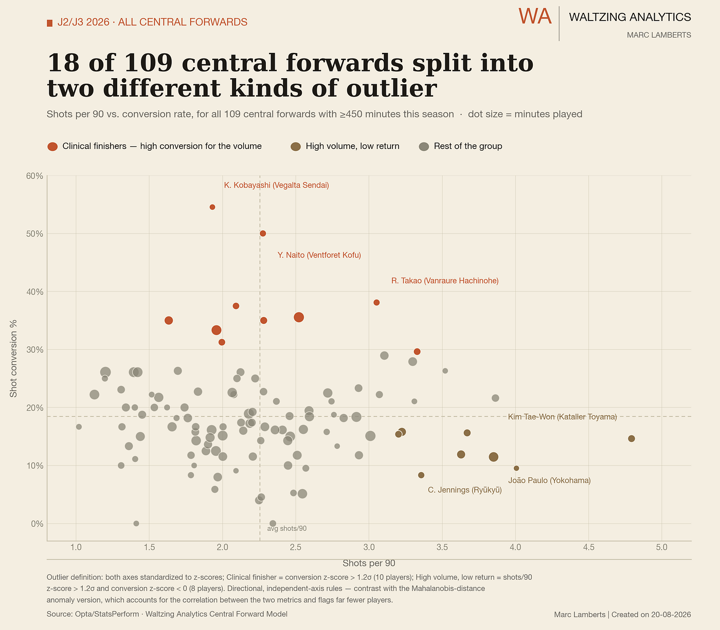
18 of the 109 central forwards (≥450 minutes) get flagged in the way with heterogeneous outliers. These are splits in outliers per metric set. You can see the clinical finisher on the top left and the high volume, low return on the bottom right.
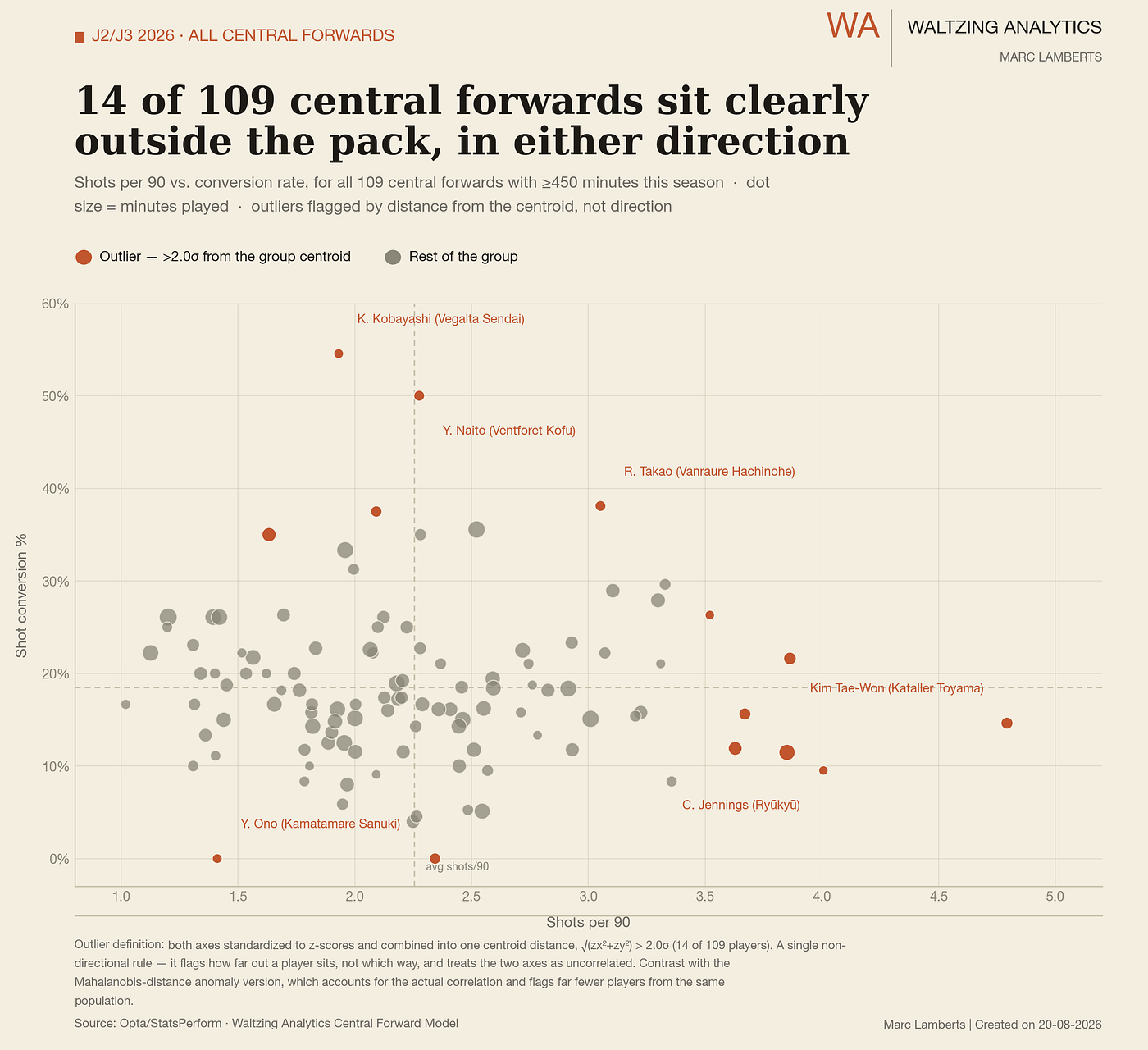
Looking at the homogeneous outliers, we see something slightly different. 14 players are selected as outliers, and they are all generated as being 2 standard deviations away from the mean.
Scouting II: Anomalies
We don’t have to run the filters again for the shots in the box and the touches in the box, because we already have that. However, we are now scouting for anomalies.
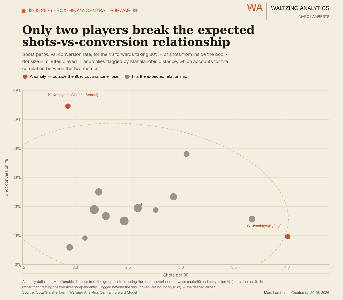
Rather than judging each player against the two axes separately, this chart measures Mahalanobis distance: how far a player sits from the group centroid once the actual covariance between shots per 90 and conversion % is taken into account (the two are mildly negatively correlated here, r = −0.18).
In practice this means the boundary isn’t a simple box or crosshair around the average, but a tilted ellipse that follows the real shape of the data: a player can be individually unremarkable on both metrics and still count as an anomaly if their combination of shot volume and finishing breaks the pattern the rest of the group follows, and conversely a player can look extreme on one axis alone and still be unremarkable once that correlation is priced in. The boundary is set at the 90th-percentile chi-square threshold for two degrees of freedom, shown as the dashed ellipse on the plot.
Of the 13 box-heavy central forwards in this group, only two sit outside it: K. Kobayashi, whose conversion rate is far higher than his modest shot volume would predict, and C. Jennings, whose shot volume is far higher than his modest conversion rate would predict. Three other players (Patric, H. Hidaka, and R. Takao) looked unusual under a simpler z-score test earlier in this analysis, but once the correlation between the two metrics is accounted for, all three turn out to be consistent with what the group’s overall relationship predicts.
But 13 is far too few; let’s go back to the drawing board and look at all the central forwards:
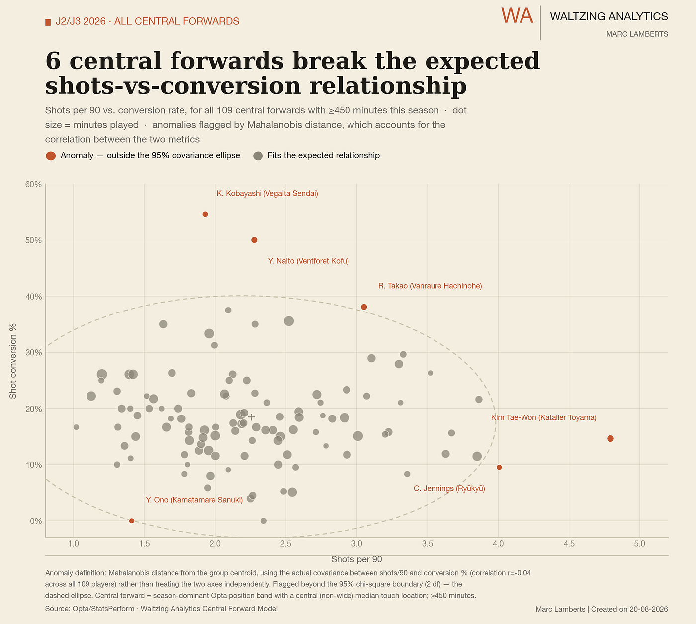
Six anomalies across all 109 central forwards (≥450 min): K. Kobayashi and Y. Naito (huge conversion for low volume), R. Takao (efficient at moderate volume), Kim Tae-Won and C. Jennings (very high volume, modest conversion), and Y. Ono (0% conversion). Note the ellipse here is nearly circular rather than tilted, across the full population shots/90 and conversion% are barely correlated (r = -0.04), unlike the 13-player box-heavy subset. This has a 95% chi-square boundary.
Final thoughts
The distinction between an outlier and an anomaly might appear semantic, but it changes how we interpret a player’s performance. An outlier is extreme relative to the group on one or more metrics. An anomaly is unusual relative to the pattern we would expect after considering the context and relationships between those metrics.
That difference matters in scouting. Outlier detection can quickly identify players with exceptional shot volume or conversion, but it does not explain why they are extreme. Anomaly detection adds another layer by highlighting players whose combination of characteristics does not fit the group’s usual behaviour. Neither label automatically means that a player is good, bad or even genuinely different. It simply tells us where further investigation may be worthwhile.