Football metrics and models are also under the influence of trends within football. One of these trends is the use of set pieces to generate meaningful chances in the game. Another big recent trend or influence on the game is the use of long balls, specifically launches. In this article, I want to have a look a this trend, but also look ahead and why long balls are used. And, why are second balls vital

Aim

The aim of this research and, therefore, this article, is to have a look at how we shape long balls and how they interact with the teams. But, even more important, we are going to have a look at what second balls are from those passes. More and more we look at what’s happening at the middle of the park: transitions and pressing are good examples.

I also want to go further than just looking at aerial duels won %: these measure the first contact, but much more important is the retention of possession. With possessions, you can actually create sequences that are meaningful towards the attack. That’s where the second balls come in.

Second balls are defined later on, but we look for second balls, as the first contact is often an aerial duel. This duel is often 50/50 and even if the header is won, the possession isn’t determined. Therefore the second ball. If a team targets long balls and loses all aerial duels but wins the second balls, they are dominant. Even if their won aerial duels percentage is incredibly low. And that’s the POV of this research.

Data explainers

I’m using raw event data, which is positional XY data. The reason why I’m looking at positional data and especially raw data is that it allows me to fully build my own metrics and models. When I use things predesigned it either hasn’t the right definition or I don’t know how it is compiled.

This is data is collected from the Opta API, and the data I collected is from the 2025-2026 Eredivisie season. This was done on the 26th December of 2025. The model I create is meant to be for educational purposes; if I was to use it, I would actually load more files into the model.

The data can be used in different formats, but I’m using JSON files to load the data and convert to my database. You can also work with CSV and Excel, for example, but the latter isn’t ideal. If you were working with JSON, you have to make sure you normalise the date before you can properly work with it.

Programming languages

I mention this every time I write an article, and you will know by now that I predominantly use Python. But I’m also well-versed in R and Julia. A good exercise for me is to create things I make with data engineering in all of the programming languages I master. It really doesn’t matter as long as you get to the result you want. If you feel more comfortable at one language over the other, go for the one you like.

What’s important, regardless, is that you know the calculations and how to structure them. If you know that, it doesn’t really matter as much which programming language you use.

Personall,y I have used Python for this one, but I’ve also used SQL to structure the database after I got the results of my model. I want to add the values to my already existing database.

Part I: Long balls

What is a long ball?

Before we are going to anything with our raw data, we need to define what we see as a long ball. Every data provider has a different way of defining it and designing it.

• When we look at Wyscout, they define it as an aerial pass that exceeds 25 meters or as 45 45-meter for a ground pass
• Opta makes a difference between long balls, chipped passes and launches. The long ball is a pass that exceeds 32 meters. The difference between a chipped pass and a launch is the intention of the end location: designed for a teammate or designed to go into a position for a player to go to.
• Statsbomb has the same distance rules, but makes a difference between unpressured and pressured balls for the long balls.

I’m working with Opta data, so I’m going to use the distance definition of 32 meters, but then the question arises: what is a long ball telling us? And should it be both targeted and untargeted? I am going for launches because it sets up for 50/50 challenges in the air, and that’s what we need. A chipped pass is a pass that’s designed to avoid opposition involvement and therefore won’t help in the second part of this article.

Methodology

The methodology behind this is that we are going to look at the raw event data and, through Python code are going to design a metric that can be used for much more. We are going to take the launches from the defensive third that exceed 32 meters and end up in the final third.

The reason why I’m going to do that is that we are seeing long balls as a tactical instrument to force attacking options in the attacking third. So what we are going to do here is see what the long balls actually are, which you can see below:

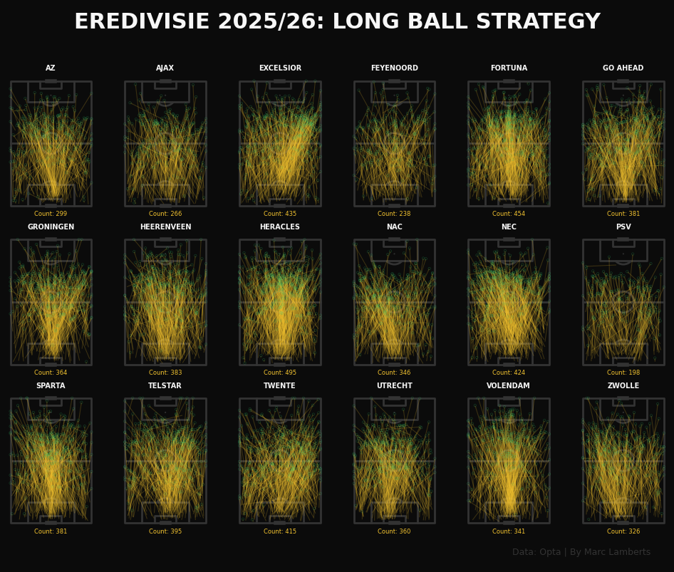
In the image above, you can see the long balls by each team in Eredivisie 2025-2026. It features the counts of these passes as well as the locations where they are. At first glance, we can see that many of these particular passes have come from the middle and from the goalkeeper areas.

The last thing we do for these passes is to see where they most frequently end up for each team. We already have the right definition for our further calculation for our model, but let’s see where most of these long passes end for our teams.

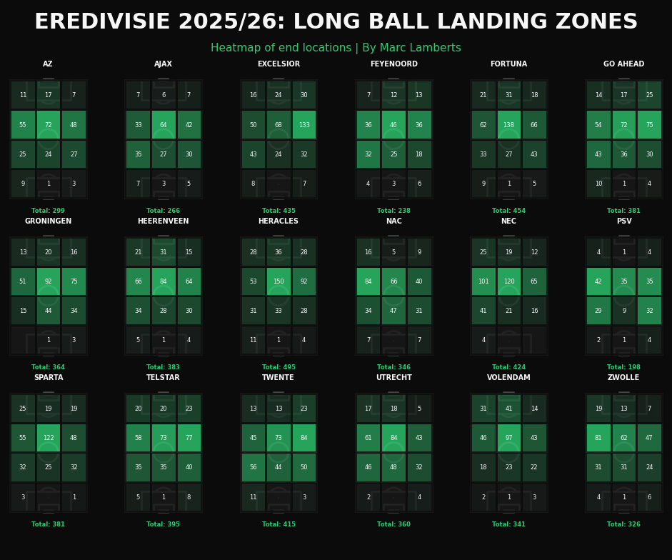
In the heatmap above, you can see the end locations of all long passes and what it shows is where most passes end, but it also leads me to a new conclusion. I might have to readjust my intention of looking at final third receptions only, but I have to look at the attacking half/opposition half. That’s where most of the passes end, as you can see from the green above.

Part II: Second Ball Retention

What are second balls?

So now we are going up to the second part of the research, which is where we want to be. First, we have to define what second balls are. A second ball refers to the moment a ball becomes loose and contested immediately after an initial aerial duel or challenge. We have to look at it as a two-stage event:

1. The first ball: A long pass or clearance is played. Two players (usually an attacker and a defender) jump to head it or challenge for it.
2. The ball is not cleanly caught or controlled. It “drops” into a space near the original challenge. The player who reacts fastest to secure this loose ball has won the “second ball.”
   
   

What’s interesting about the second ball as well is the uncertainty. We can have end locations for passes and therefore the location of aerial duels, but we cannot really predict where the ball will drop before the second ball is regained. We speak of the drop zone, which is often 10-15 meters in radius from the pass end location. It focuses more on anticipation than raw skill.

Having concluded that, we need to conclude two different things going forward. There is a lot of uncertainty involved in second balls and that there needs to be ball recovery or a pass within 2-3 seconds after the initial aerial duel.

Challenge: no tracking data

I don’t have tracking data available for this model, which is a challenge. The challenge here is that with tracking data, I could see how packed an area was when the aerial duel was conducted, the distances of players and how quick the reaction time was.

I can only see/detect who won the ball, but not how they won it. Is it because of better access? Shorter distance? Being quicker? I can’t do that at this point.

Since we can’t see the off-ball movement, we focus on event proximity, which calculates the spatial distance between a long ball landing and the next recorded action. If a launch is followed within three seconds by a ball recovery, a tackle, or a foul in that same 15-meter “drop zone,” we can statistically infer a successful second-ball win.

Methodology

Above, we have seen how we can look at second balls and how we can see retention from a second ball. We need to look at a few variables before we can make the calculation. First of all, the long ball should be followed by a 50/50 aerial duel. The next step is to see whether the taker of the long ball (the team that is) also wins the second ball, regardless of the outcome of the aerial duel. We will measure this by looking at the next event, which is a ball recovery or a pass from the same team. If this happens, we can state that this is ball retention.

Results

So, how can we now see what this looks like? In other words, for every team in the Eredivisie, how often do they win the second ball and therefore keep possession via the second ball?

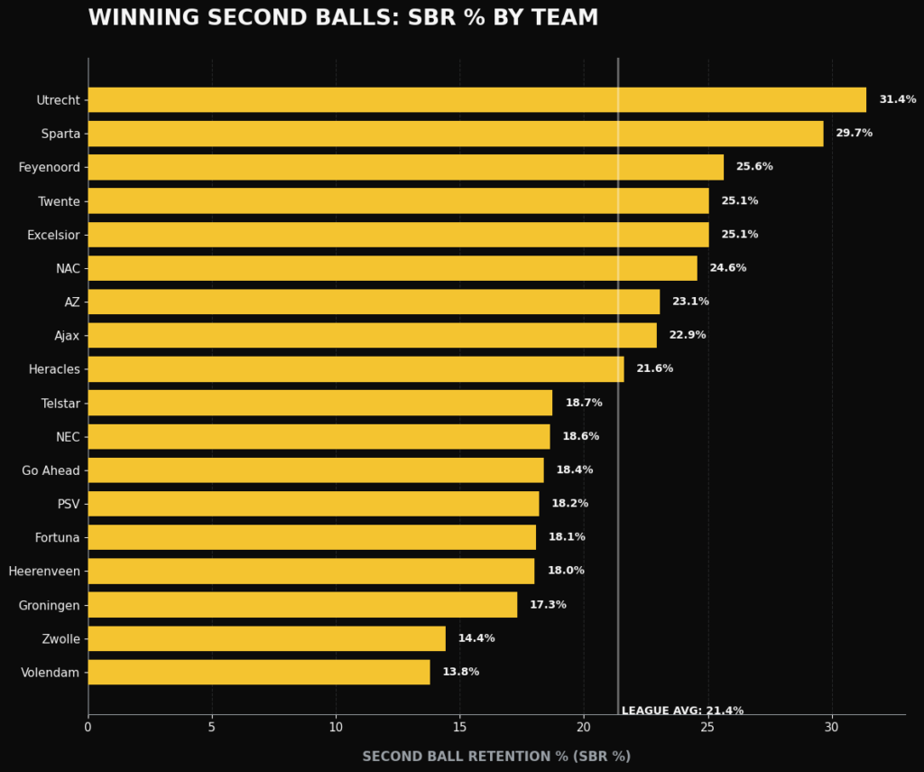
As you can see in the bar graph above, we can see how every team performs on this new metric. FC Utrecht scores the highest, followed by Sparta and Feyenoord. FC Groningen, PEC Zwolle and FC Volendam score lowest.

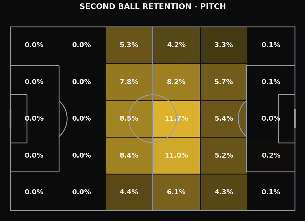
In the pitch map above, we can see the locations of where the second balls by the teams in the Eredivisie. This gives us a more clear idea of where they mostly happen and where. We have to concentrate in terms of long balls. What’s evident is that most the second balls happen in the attacking half, but more in the middle third than in the attacking third.

Lastly, we can also have a look at how the long balls line up against the second ball retention in this scatterplot below:

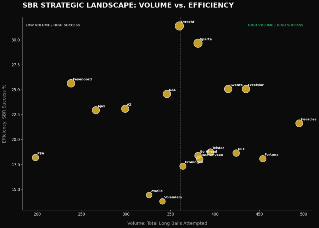
In the scatterplot above you can see how the teams perform in the long balls attempted vs the second ball retention in percentages. Heracles Almelo, Fortuna Sittard Excelsior, NEC Nijmegen and FC Twente have the highest volume of long ball.

In terms of winning second balls, FC Utrecht and Sparta Rotterdam are the clear leaders, followed by Feyenoord, FC Twente, Excelsior and NAC.

Part III: Expected Second Ball Retention (xSBR)

So, now we have defined the new metric of second ball retention. This, however, is based on historic data and actual event. What we want to achieve in the end is the Expected Second Ball Retention (xSBR). In other words, we want to add a xSBR value for every long ball from the defensive third.

To do so, we have to look at a few different things:

• Giving weights or rewards for certain zones: wide areas, half spaces, central areas, cutback zones, hot zone/zone 14/assist zone
• Giving weights or rewards for distances and angles
• Add a defensive proximity multiplier/score
• Add an entropy model for uncertainty -> without tracking data + the unpredictable nature of an aerial rebound, we need to add a factor for uncertainty
• Create the model in logistic regression or XGBoost
• Train the model 80/20 on historical data for more than just 1 season

First, we will look at giving rewards for certain zones. This seems quite straightforward by giving different weights, but we also need to make a distinction between the zones where the first contact is in (aerial duel) and the zones where the second ball is regained. The ratio for me is 3 times the importance for the second balls and 2 times the importance for the aerial duels.

Next what we will do is eaxtly the same, but for distances and angles. This will give different impacts. Distances will be the distance between the location of the aerial duel and the next event (second ball). For angle, we look at the angle from the second ball to the middle of the goal.

At this point we have this that is part of our calculations. The next part is to add a proximity score. This is needed to estimate the proximity of defenders as we don’t have any tracking data or off ball data, that will be helping us. We are going to infer proximity with our event data.

How we are going to do that? We are going to look at the second between the events. We want to look at the event of an aerial duel and see how much time it takes, before the second ball event happens in this particular sequence. If the second ball event happens in 1.5 seconds or less, we can assume that it’s a zone/situation with traffic. If the second ball event happens from 1.5 to 3 seconds, we can infere that there is room to breathe and that there is freedom. It’s about recovery speed and the window of opportunity it presents.

The last things we do before creating the model is to look at entropy. With entropy we measure the uncertainty of the outcome of the data: is it predictable yes or no, and adding randomness. We want to do this, because we don’t have the tracking data to ensure this. By adding this we help this challenge and offer a stroke of “luck” and uncertainty, which is vital.

We define low and high entropy for both the long ball start locations, as well as for the second ball recovery locations. We can develop a matrix with them. Important here is to stress that low entropy means a high predictability while high entropy mean a low predictability.

Creating the model

After running the calculation for the adjusted SBR scores, with all the weights and valuations for zones, angles, distance, proximity and entropy, we get this:

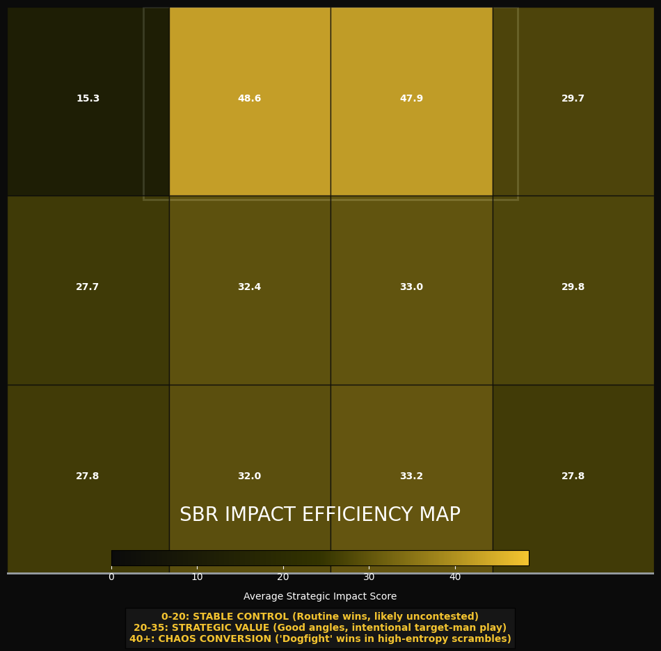
Now we have our adjusted-SBR impact. So we can establish the impact of the second ball won after a long ball and first-contact of aerial duel. This forms the basis of our expected model.

First of all we need much more data, so I will add three other seasons of Eredivisie data too: 2022-2023, 2023-2024 and 2024-2025 too. This data is needed to make the model more likely to be accurate. I will be using XGBoost over Logistic regression, because I’m working with many variables, especially weights and scores included as well.

XGBoost works through a process called Gradient Boosting. Unlike “Random Forest,” where trees are built independently in parallel, XGBoost builds trees sequentially.

• Tree 1: Makes a baseline prediction. It will likely have a high error rate.
• Tree 2: Specifically focuses on the mistakes (residuals) made by Tree 1.
• Tree 3: Focuses on the combined mistakes of Tree 1 and Tree 2.

This continues until the model minimises the error as much as possible. It is like a coach watching video footage: instead of telling the whole team to “get better,” the coach identifies the specific players who missed tackles and creates a drill just for them.

What does the model say when we load this first half of the 2025-2026 season?

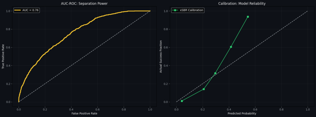
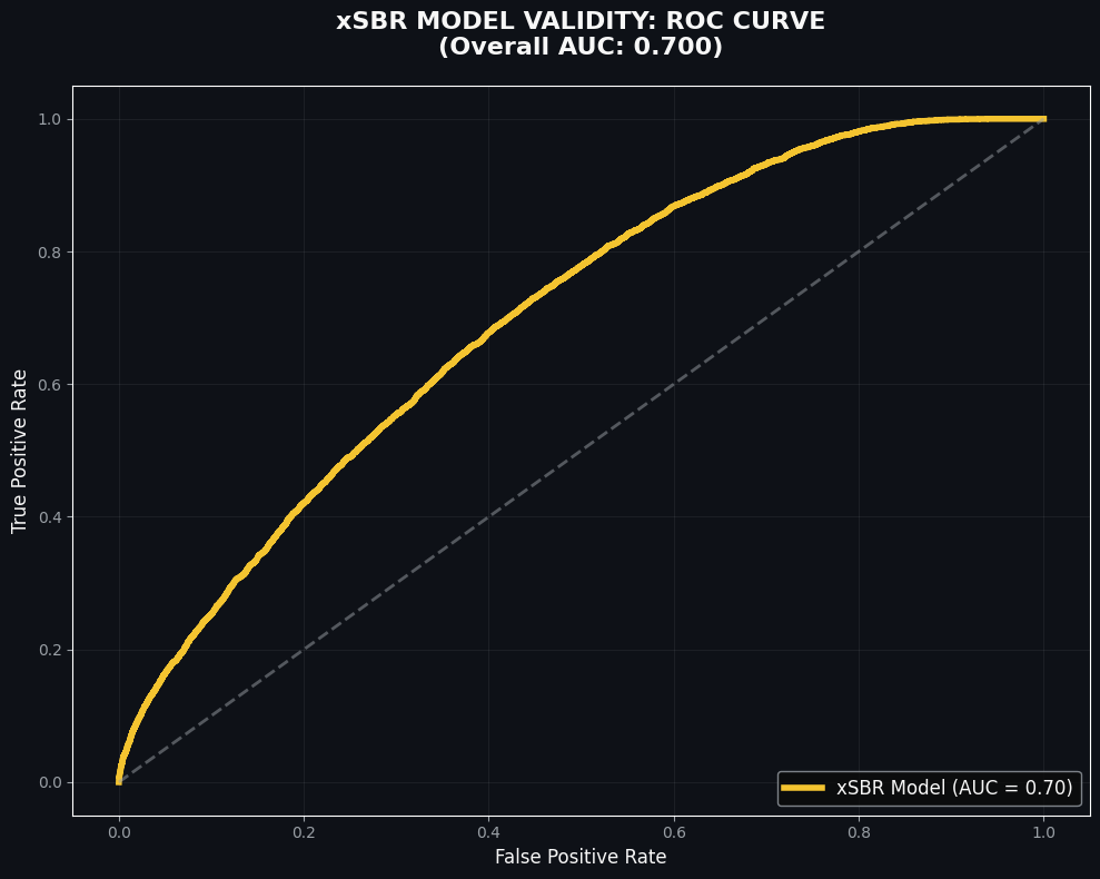
The xSBR model achieved an AUC-ROC of 0.76, indicating a high degree of predictive reliability. The model successfully filters out ‘statistical noise,’ allowing us to isolate genuine tactical over-performance from random chance. 0.76 means that if we randomly picked one successful retention and one failed retention from our 100+ files, there is a 76% chance the model would correctly identify which one was which.

We also see in the calibration that the model doesn’t go beyond the predicted probability of 60%, which can be attributed to the fact that the model right now seems to rely on easy long balls, as most of the probabilities lie between 30 and 60%. We look at the second ball retention and now in many cases, it exceeds 60%.

We can do two things now: load more data to train the data and change our features a little. First let us see how it looks like when we load more seasons:

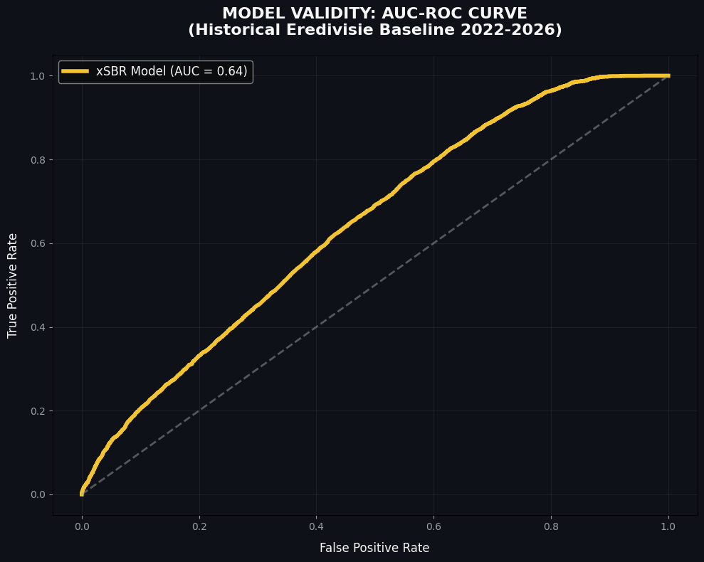
When we load the multiple seasons we can see that the AUC value has dropped to 0,64. The model has dropped from a good predictive model to a standard or even weaker model. How is this possible? This can be because of the calculations, but it can also happen because of factors within the league.

1. This can happen due to players moving and coming into the league that influences the model
2. The way teams press after an aerial duel has changed, so that results can have effect.
3. The influence of luck, randomness and individual duels

Let’s see how that looks, season per season:

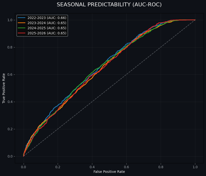
With our new calculations, we see that the score is around 0,65/0,66 every season, which likely has to do with the difficulty of prediction events due to a set of variables we have not set as features. We can improve this by changing a few features regarding predictable independence on the angle (known before endlocation), launch entropy (chaos before the pass is being taken) and the aim of the kicker.

When we add these to the model we get a more accurate idea of the predictability.

It recognises that while we can predict some success, about 30% of second-ball retention is down to pure individual dueling and the “chaos” of the bounce. This is an improvement of 4-5% and can be a good way of identifying the expected second ball retention.

Results

Now we have saved the model and used that model to convert the data by the current season. This give us a different perspective on actuals and expected data, especially since we still have that chaos included in our results.

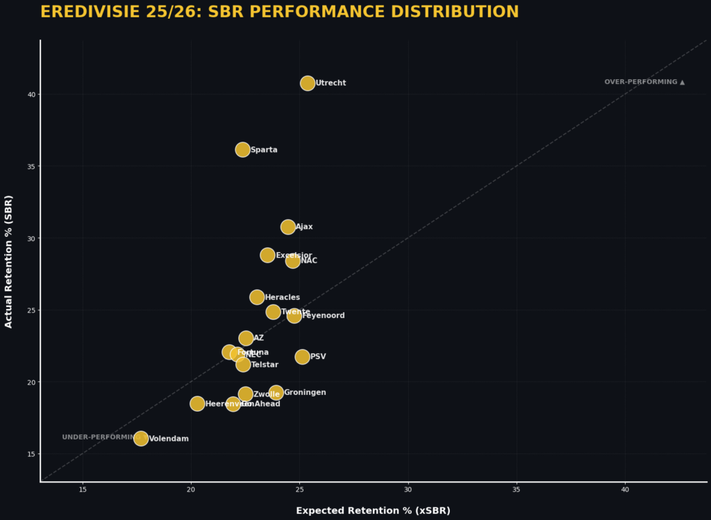
In this scatterplot, you can see all teams in the Eredivisie 2025-2026 and their results. You can see that in general, most teams stay around the right calibration, but there are some outliers in doing so. The chaos and unpredictable nature makes it so that we will stay away from higher predictability, but it still gives us an idea of the team’s indications.

What else we can create is to see a distribution plot, so we can see what the most common values are connected to our specific long balls:

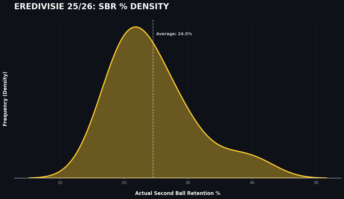
Here you can see that the most percentage for the second ball retention are between the 20% and 25%. The average of the second ball retention % for long balls sits on 24,5%. This is interesting, because it gives us the indication that 1 in 4 long balls, has a second ball retention for the team taking the long ball..

How does this look for the expected side of it?

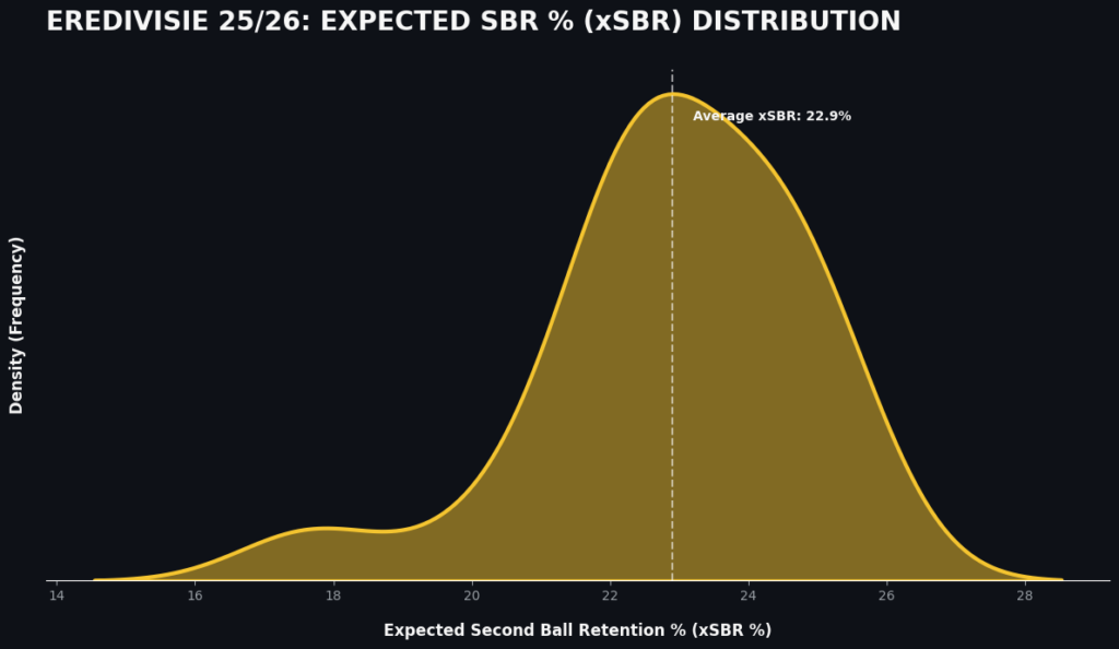
This looks a bit different too the second ball retention %. The average is 22,9% and that’s not very much difference to the actuals. The distribution however is concentrated between 21 and 24, with a maximum of 28%. This is a big difference with the actual have a maximum of 50%.

The significant delta between the maximum (50%) and Expected SBR (28%) indicates that Eredivisie teams in the 2025-2026 season are exhibiting high tactical efficiency and superior individual duel-winning capabilities. The model provides a physics baseline (28%), meaning that the remaining 22% of retentions are a direct result of coaching structure and player quality rather than the ease of the pass itself.

New metrics

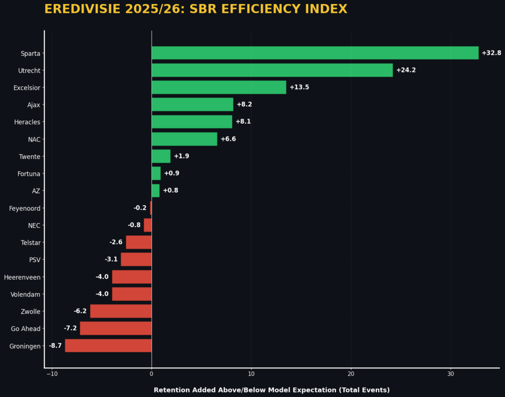
1. SBR Efficiency Index (Retention Added)

SBR Efficiency Index measures the side’s relative strength to exceed the probability of the match. Subtracting the cumulative Expected Second Ball Retention (xSBR) from the total Actual Retentions helps filter the value created by the playing and coaching staff. In such a context, it shows that when the Efficiency Index is also positive, it states that their team is equipped with better aerial duel participants or that their structural pressing trap is highly disciplined in terms of “loose” ball recovery, exceeding the mean rate in their league.

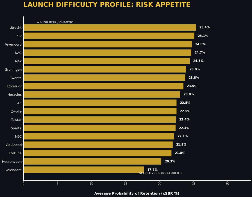
2. Launch Difficulty Profile (Risk Appetite)

The Launch Difficulty Profile is a strategic signifier of a team’s distribution philosophy rather than a metric of success. It plots the average Expected Value of the passes being made. A lower Profile indicates a ‘High Risk’ approach, where there is a penchant to launch the ball into dense, high-entropy areas, often resulting in a physical contest. A higher Profile indicates a ‘Selective’ distributor, who makes use of long verticals only when structural angles indicate a high chance of successful, uncontested recovery.

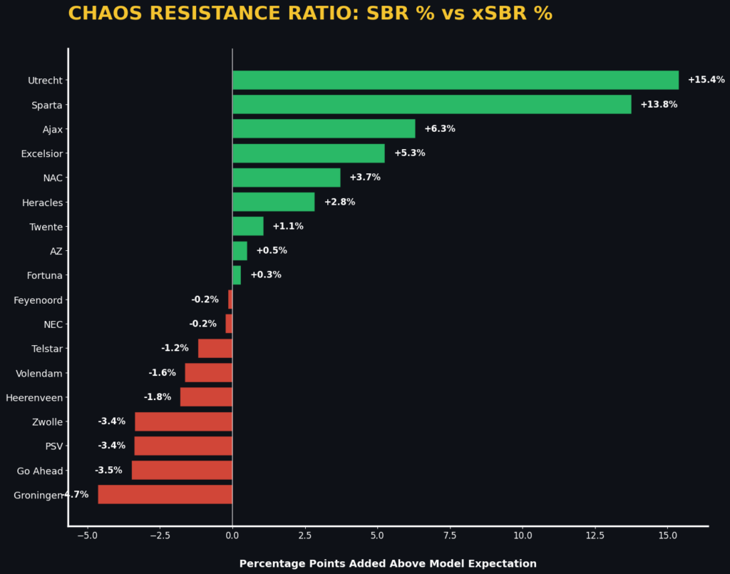
3. Chaos Resistance Ratio (High-Entropy Dominance)

The Chaos Resistance Ratio in isolation performance in “Broken Play” scenarios specifically filters for events with an xSBR of less than 20%. In these high-entropy instances, the ball is objectively “50/50” or worse. Teams with a high Ratio in this category demonstrate systemic resilience to randomness, evidencing a team that thrives in the “scramble” phase of the game. This would be an essential metric for recruitment and scouting as it would identify squads that can maintain possession and territory in high-pressure match scripts where clean tactical structures have broken a vital trait for success in knockout competitions and high-intensity derbies.

Best players that lead to second ball recovery

Now we move one from teams to players. I want to know what the best players who start the long ball, as first.

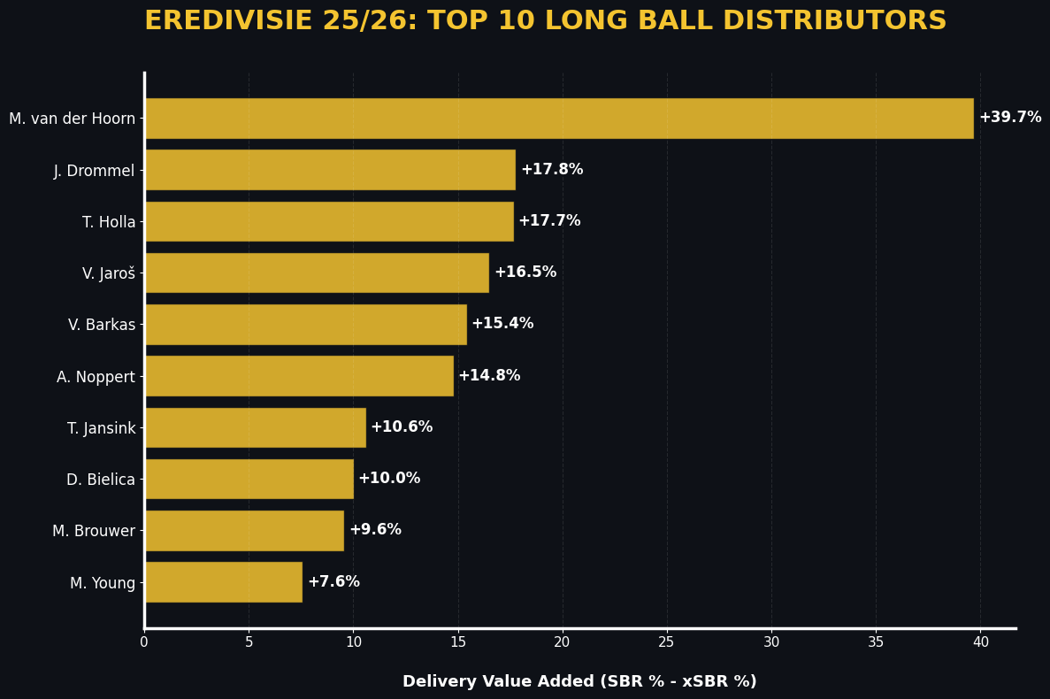
In the bargraph above, you can see the players whose long ball lead to the highest value added in terms of second ball retention. What’s interesting is that most of these players who rank high are also from the goalkeepers’ rank, but M. van der Hoorn just stands out from the crowd.

So let’s look a step further, which players wins the most second balls?

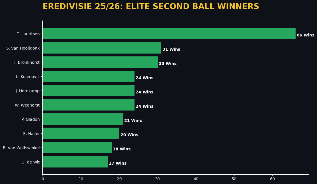
Here we see the players who win the most second balls. Lauritsen is an exceptionally good second ball winner, followed by Van Hooijdonk and Brinkhorst.

What we can do with this data is anticipate in which areas second balls are most likely to be won, and have a look at which players we want to target. The second ball winners don’t necessarily have to be the ones with the aerial duels, but it’s important that we have them in and around that area. This makes this theoretical framework actionable for football coaches.