Expected goals. I don’t even know where to start with how I feel about this particular metric, but I’m going to try it anyway. I feel that expected goals are actually an exciting metric and concept, but it’s more complex than popular sports media often portrays. And, I think that’s primarily because we don’t fully grasp what it takes to create such a model. That’s exactly where it does pique my interest, but in a different way than you might expect.

Creating an expected goals model is something I’ve already done, and making such a model really makes you appreciate what complexity lies behind it. This article aims to show two different things:

1. What goes into creating a shot-based probability model?
2. In what way can we create an alternative to expected goals?

It’s important to stress, however, that this isn’t an expected goals model — but an alternative which can measure the same thing. This is called the Expected Shot Danger model.

Contents

1. Data explanation and justification
2. Concepts from the NHL
3. Theoretical framework: Probability models
4. Methodology: Python
5. Calculations
6. Model results
7. Applications
8. Final thoughts

Data explanation and justification

The data used for the creation of this model is from Opta/StatsPerform. I have used raw event data — which is XY-positional data — to calculate it all. This gives me the freedom to do what I want. You can use other data providers, of course, but be aware that this is a conscience decision and that a choice for a certain data provider also comes with its own pros and cons. Also, it’s good to remember that while people talk about data being unbiased and objective, it never is. Every decision you make in terms of building/handling the data in this model means that it is biased. Whether that’s good or bad is a whole different question altogether.

Every model has to be created, but it also has to be trained. This means that enough data has to be imported and used. To just train it on a single season of a single league won’t paint a representative picture. That’s why I have trained in three different seasons for the following leagues:

• Eredivisie (NL)
• Eerste Divisie (NL2)
• Pro League (BEL)
• Premier League (ENG)
• Eliteserien (NOR)
• Allsvenskan (SWE)

This will be different from different leagues, obviously, but in the end, the result can be used across all the leagues. My own xG model has been trained on 500,000+ shots on a single league and is pretty accurate for other leagues too.

The data was collected on December 10th 2025, via the Opta API. The model is an update from an older model I have already created. This actually is version 4.2.1 and is evidence that it takes time and effort to create something you are comfortable with.

2. Concepts from the NHL

I learn a lot from data concepts from other sports, and for this model, I look to Ice Hockey data, the NHL in particular. They have a particular way of evaluating shot data with Fenwick and Corsi, which will be instrumental to my model. The definitions will follow below.

2.1 Fenwick
Fenwick is an unblocked shot-attempt metric that counts shots on goal and missed shots while excluding blocked shots. By removing blocks, which often reflect defensive structure more than offensive intent, Fenwick isolates attempts that genuinely reach or approach the scoring area. This makes it a cleaner indicator of how frequently a team produces potentially dangerous opportunities.

Fenwick is used because unblocked attempts correlate more strongly with sustained offensive pressure and long-term scoring performance. Over larger samples, teams with higher Fenwick percentages typically demonstrate more consistent puck possession and shot-quality generation. As a result, the metric serves as a practical tool for evaluating underlying play beyond what the scoreboard or raw shot totals reveal

2.2 Corsi
Corsi is a shot-attempt metric that includes all attempts toward the net: shots on goal, missed shots, and blocked shots. It captures the total volume of offensive activity by tallying every attempt a team generates or allows, providing a broad measure of territorial control and play-driving ability.

Corsi is used because shot-attempt volume is strongly associated with puck possession and long-term team success. Although it weighs all attempts equally, its comprehensive nature makes it a stable predictor of future performance. Teams that routinely out-attempt their opponents tend to control the flow of the game, making Corsi a foundational metric for modern hockey analytics.

This distinction is very important to me as it forms the basis of my expected shot danger model. I include blocked shots, and therefore we can assess more about shot danger.

3. Theoretical framework: Probability models

So why do I do this, and what’s my aim? I aim to create a shot-based value model that is a hybrid between expected goals and expected threat that seeks to measure outcome danger whilst including blocked shots.

The model is designed to overcome a key limitation of existing football analytics models. It combines the strengths of two popular metrics:

• Expected Goals (xG): This model calculates the probability of a shot resulting in a goal based on factors like shot location, body part used, and play type. Its primary focus is on the final outcome: a goal. However, it assigns a value of zero to shots that are blocked, even if the shot was taken from a high-danger location.
• Expected Threat (xT): This model measures the change in a team’s probability of scoring when the ball moves from one location to another. It values passes and carries that move the ball into more dangerous areas, but it doesn’t directly value the shot itself.

What’s important to know about the theoretical framework, however, is that this is a model that calculates probabilities based on historical data. After that, we can use the model to calculate probabilities for more recent games and assign expected shot danger values to shots and players, and teams.

4. Methodology: Python

In the past few years, I have been developing expertise and interest in different programming languages to work with data. For the creation of the model, I have chosen Python over other languages such as R and Julia. The reason for this is that I am simply better at writing Python code, and I know what to do for these kinds of advanced models. That’s not to say you can’t create this in other languages, but that’s simply what I’ve been using. But I will also list some of the key Python packages I’ve used to create the model and some of the visualisations (however, I think ggplot in R also creates great data visualisations).

4.1 Matplotlib
Matplotlib is a widely used Python library for creating static, animated, and interactive data visualisations. It provides fine-grained control over plot elements, allowing researchers to customise figures to match academic or publication standards. The library supports a broad range of chart types, from simple line and bar plots to complex multi-panel figures. Because of its flexibility and stability, Matplotlib serves as the foundational plotting tool in the scientific Python ecosystem. Many other visualisation libraries build on top of it or integrate seamlessly with its framework.

4.2 Numpy
NumPy is the core library for numerical computing in Python, offering fast and memory-efficient operations on large multidimensional arrays and matrices. It provides a wide range of mathematical functions that operate at compiled speed, enabling efficient data manipulation and analysis. NumPy’s array structures form the backbone for many other scientific libraries, including pandas and scikit-learn. Its ability to vectorise computations allows researchers to avoid slow Python loops and write concise, high-performance code. As a result, it is essential for any workflow involving numerical data.

4.3 Pandas
Pandas is a data manipulation and analysis library built around flexible data structures such as Series and DataFrames. It offers powerful tools for cleaning, transforming, merging, and aggregating datasets, making it especially useful in data-heavy research workflows. With its intuitive syntax and built-in handling of missing values, pandas simplifies complex data operations that would otherwise require extensive coding. It also integrates smoothly with libraries like Matplotlib for quick visualisation. Pandas has become a standard tool for organising and preparing data prior to statistical analysis or modelling.

4.4 MPLsoccer
MPLsoccer is a plotting and analysis library designed specifically for soccer analytics, built on top of Matplotlib. It provides ready-made tools for creating pitch diagrams, tracking visualisations, passing networks, and other soccer-specific graphics. The library streamlines the production of publication-quality sports analytics figures that would otherwise require extensive custom plotting code. MPLsoccer also integrates well with pandas and NumPy, allowing analysts to move easily from data preparation to visualisation. Its domain-specific functionality makes it a preferred toolkit for researchers and practitioners working in soccer data science.

5. Calculation

The first thing I do is look at my data. I have JSON files rather than CSV files, purely because it’s easier to work with, and that’s how I save them. That means that we need to load them into our Python code and handle them as such, otherwise, it will be difficult to make the right DF (=dataframe). I will filter for shot events only:

• typeId = 13 -> Missed shot
• typeId = 14 -> Shot on post
• typeId = 15 -> Shot on target
• typeId = 16 -> Goal

I filter for these events, and they come with their own qualifiers and XY-coordinates, which will be proving important for actually building the model. Now I want to add a specific shot, which is the blocked shot. As I previously mentioned under the NHL data analytics part, I want to incorporate the danger of the blocked shot through this dataframe/model as well.

Then we look at shot context and mathematical physics-based features. Within the context we look at:

• body part used
• type of play (open play, counter, set piece, penalty)
• shot technique (volley, chip, overhead, etc.)
• assist type (cross, through ball, pullback, etc.)
• whether the shot was deflected

This gives us different qualifiers from the data. To add to the calculation is what I like to call distance and angle-based features: distance to the centre of the goal, shooting angle and variations of the two.

Fenwick and Corsi are indications of strong attacking performance/weak defending performances as to the danger that comes forth from (un)blocked shots in our dataframe. This is important as to why it differs from typical xG.

The last part of the calculation is a two-stage process of making this model. In stage 1, we predict the probability that a shot becomes on target. This isolates the ability to reach the goal. In stage 2, we predict the probability that an on-target attempt becomes a goal, based on shot quality.

Expected Shot Danger = P(on target) × P(goal | on target)

This mirrors how goals happen in reality:

1. A shot must first be directed well (accuracy)
2. Then it must beat the goalkeeper (finishing quality)

To do all this, I employ 4 different models:

1. Logistic stage 1 model
2. Logistic stage 2 model
3. LightGBM model: A highly efficient, modern gradient boosting framework that uses a novel technique called Gradient-based One-Side Sampling (GOSS) and Exclusive Feature Bundling (EFB) to train faster and consume less memory than traditional boosting models like XGBoost.
4. XGBoost model: A highly popular and powerful optimised distributed gradient boosting library designed to be extremely fast, flexible, and portable, known for its regularisation techniques to prevent overfitting and its success in predictive modelling competitions.

And, out comes my model saved in PKL files.

6. Model Results

Okay, not the desired result is still a result, right? At this point, I first created a model solely focused on the Eredivisie 2025–2026 to give it a trial run. To assess my probability models, I use a ROC-AUC curve. This measures the ability to identify positive and negative rates of the model. Positive rate measures the ability of the model to identify positive rates, while negative rate measures when the model identifies negative rates as positive. It’s measured between 0–1, and the higher the number, the better the model performs. It’s an indication of my ranking probability quality.

So first run with only one season in one league:

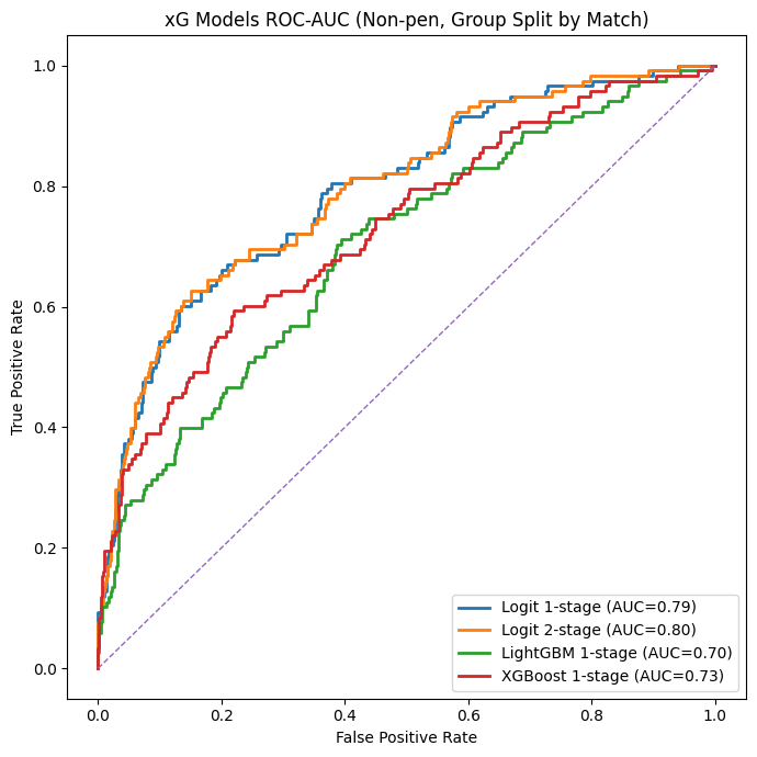
In the visual above, we can see how the AUC scores. The logit 2 stage model scores the highest with 0,80, which is an excellent score; the logit 1 stage has 0,79 very good as well. LightGBM and XGBoost score lower with 0,70 and 0,73. However, this is just based on a single season in one specific league.

What happens if we load multiple leagues? How does the model change?

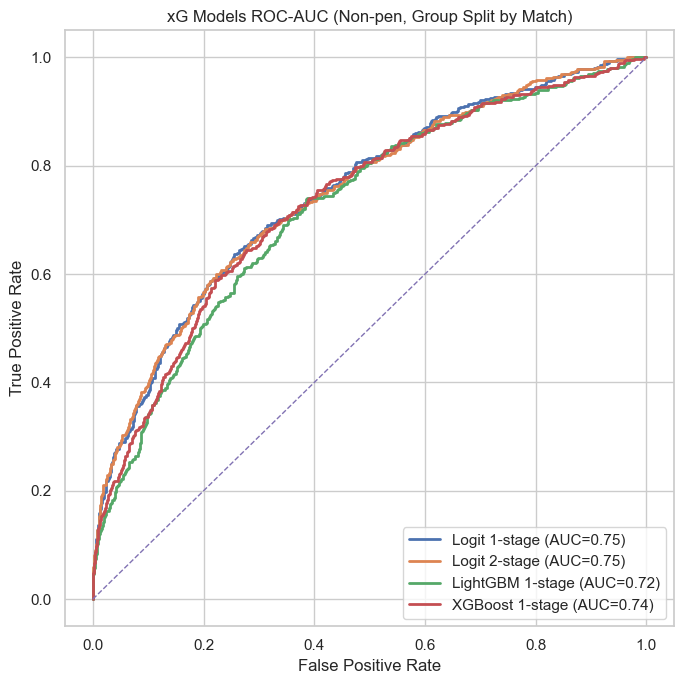
So as you can see, things are completely changing from loading all of our leagues. It’s evident that the AUC-scores will be lower, and what we see is that the differences between the scores are still closer to each other. I like this a lot better overall. I can go on and work with this.

I realised something midway through my next model: this is just an expected goal model with a slight modification. Yes, I want to create an alternative to the expected goal model, but I primarily want to capture shot danger.

Instead of calculating the goal probability, I’m going to calculate the probability of a shot on target as a pre-shot danger model, and the probability of a shot on target being a goal with a post-shot danger model. Having done that, we get the following curve:

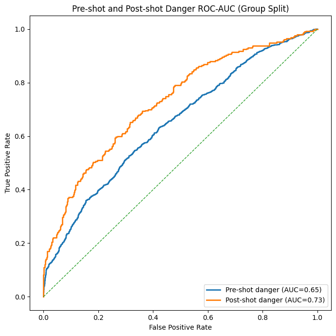
As you can see, I switched from how I created the model, which focuses on pre-shot and post-shot danger. The AUC is lower on the pre-shot, but that is also due to the fact with much more variables and uncertainty. This is the model I’m using to go to the application of my work.

7. Applications

Now, we are going to use it. What can we do with it, and what kind of visuals can we portray? First of all, we can look at the distribution of our new metric: Expected Dange,r in both models:

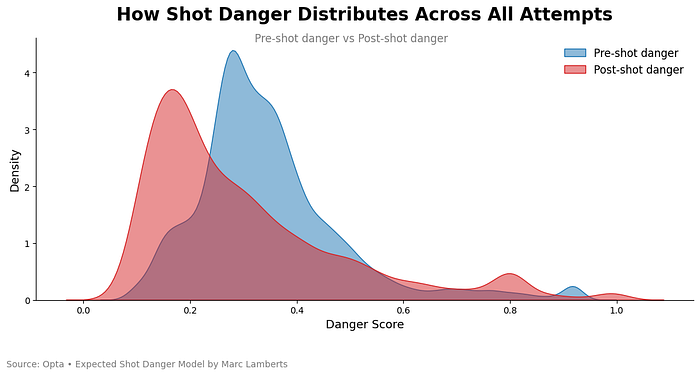
What we can analyse is that there are more lower danger score shots in the post-shot model than there is in the pre-shot model. However, there is more high post-shot danger than in the pre-shot danger.

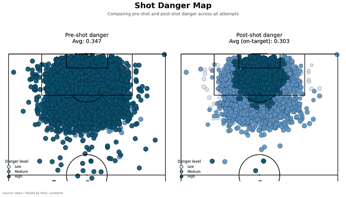
In the above shot map, we can see how they compare to each other in terms of the models. Pre-shot danger averages higher, but we can also see where the average on target danger comes from; it’s much more concentrated closer to the goal.

Another area of application which is interesting is the blocked shots vs unblocked shots.

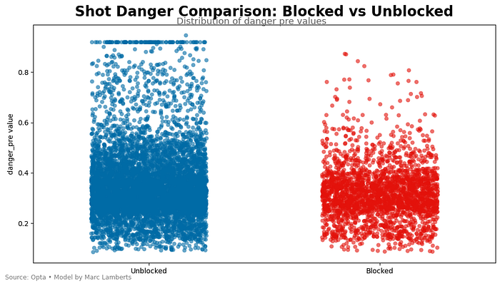
Here we can see that there are fewer blocked shots and with lower values, but the majority of the blocked shots still have a consistent value. And some have a high value still, which indicates that block shots are associated with danger. Something you wouldn’t see in traditional expected goals.

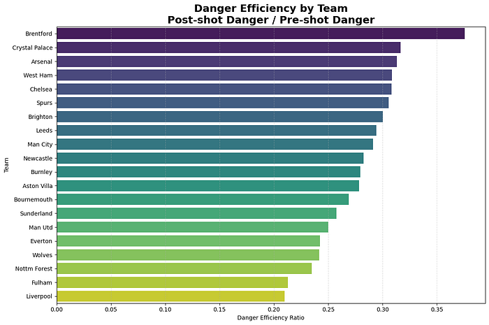
Here we can see that Liverpool has the greatest total danger of shots, but their post-shot danger value shows us that there is a big difference in how their dangerous shots actually become a threat. Manchester City, Arsenal and Brentford score the highest on their post-shot danger levels.

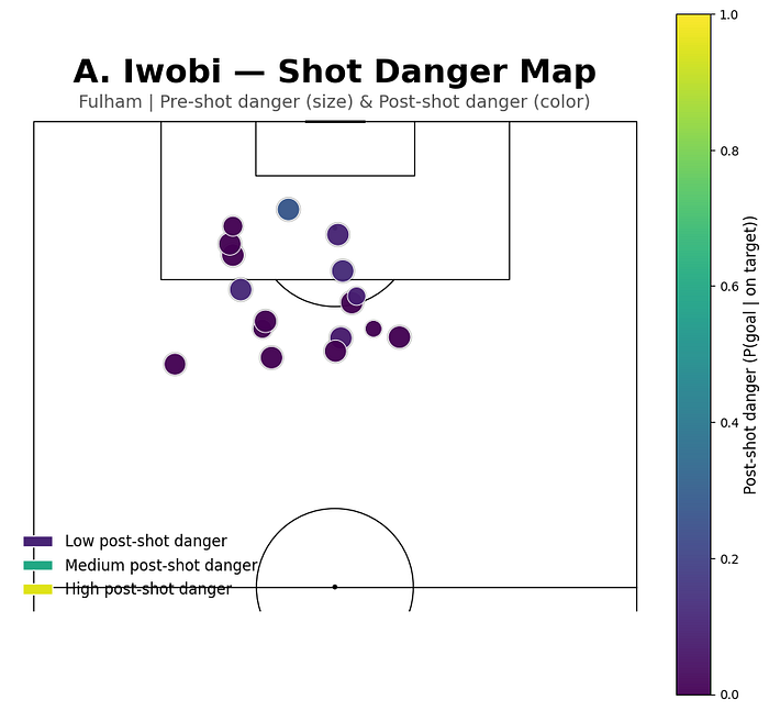
Let’s take a step closer towards player level as an example and look at a few players.

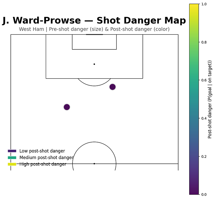
Final thoughts

The pre-shot and post-shot danger model offers a clearer, more decomposed view of finishing quality than traditional xG. By separating the likelihood that a shot becomes dangerous (reaching the target) from the likelihood that a dangerous shot becomes a goal, the model exposes two distinct skill sets: creating clean shooting conditions and executing decisive finishes. Even with event data alone, features such as location, open angles, technique, assist type, and team shot tendencies provide enough structure to produce stable patterns that align with football intuition. The resulting danger maps and distributions reveal meaningful differences in player profiles, team attacking styles, and defensive disruption effects that xG alone tends to compress.

At the same time, the model highlights the inherent limitations of event-only data: it lacks defender pressure, goalkeeper positioning. Still, the framework’s biggest strength is its modularity. Each stage can be refined independently, swapped for more advanced models, or expanded with new features.