
I will be honest with you. This article is a passion project of mine and it combines two things I really like in football: data and dribbles. I get it, this is ridiculously vage and broad, but hear me out. There is something magical about a 1v1, a take-on, a dribble or a carry. A player with the ball on their feet, trusting vision, ability and pace to make something meaningful out of that situation. It’s a form of arts and its beauty is perceived differently by anyone looking at it.
So how does this relate with data? Again, I do understand that you might anticipate that I won’t only look at regular aggregated data and you are totally right. After spending my time on Jstor reading about sports analytics (100 free articles per month btw, you are welcome) – I became fascinated with several statistical concepts and one of them is the Hidden Markov Model in sports analytics. I didn’t trust myself to look at it too much, because of two reasons.
The first reason is simply that I didn’t understand it enough to apply it to football. How was I going to be able to convey this methodology to football and make it meaningful? The second reason was the one that followed that thought pattern: football is much harder to grasp than others sports, because there are so many *states*, but more on that later.
This piece will be long and explanatory, maybe a little bit on the heavy side. But I will take you along on the journey of me trying to find out the mathematical and statistical side of it, as well af the pure footballing data side.
To begin at the beginning…
I think it’s important to answer a question before I go into the contents of this piece. The general question around every piece that I write: **Why do we need this article and this specific data analysis?**
Is the question of needing the right one? I don’t think we really need it, but I do think that’s good exercise to know what data can do with dribbles and their next actions, to see what we can learn from high volume data. If we can analyse full seasons, that will lead to more value of data, which we can make actionable in a later stage. So, long story short – it can help us value dribbles and their sequnces to see where and how the most value is added.
Next to that it gives a bridge between tactics and data. Hidden Markov Models deal with states rather than action, and in this context these states can be tactical states. We can learn whether a dribbles lead to progression, chance creation, retention or defensive state. But more on that later.
Contents
1. Data collection
2. Glossary
3. Theoretical framework: Hidden Markov Model
4. Methodology: from data to hidden states
5. Analysis
7. Case Study: Most attacking players in Premier League
8. Challenges and difficulties
9. Final thoughts
10. Sources
Data collection
I always start the articles with this section, but it’s vital to know where and how we collect our data. The providers are different and therefore outcomes can be slightly different as well. For this research I’m using Opta/StatsPerform data from the Premier League 2025-2026 season so far. The data has been collected on September, 17th 2025. I’m working with event data rather than aggeregated data, because the raw positional data (X,Y-coordinates) give me the relative freedom to design metrics and models to my own liking.
As far as changing the data, and with changing I mean manipulating, I’m not doing a lot at the first stage of this research. The only thing I’m doing here is look at end locations. The end locations of passes or dribbles are not automatically in the data, so that’s the first thing I do. I look at qualifiers 140 and 141 for endX and endY for passes. Endlocations of dribbles can’t be drawn in the same way, but I will calculate them by look at the next action and use that specific XY-coordinate to determine this.
Glossary
I am not going to give you the full glossary here, if you are interested in that you can visit this website by StatsPerform that explains most of the uses metrics. I want to focus on what’s central in our research, dribbles:
“This is an attempt by a player to beat an opponent when they have possession of the ball. A successful dribble means the player beats the defender while retaining possession, unsuccessful ones are where the dribbler is tackled. Opta also collects attempted dribbles where the player overruns the ball with a heavy touch when trying to beat an opposition player.”
Using this, we will conduct our further research into dribbles and dribbled modeling using Hidden Markov Models.
Theoretical Framework: Hidden Markov Models
A Hidden Markov Model (HMM) is a statistical model that represents systems where we can observe some data, but the underlying states that generate this data are hidden. Unlike a simple Markov chain, where the states themselves are directly visible (like “hot” or “cold” weather), an HMM assumes that the states are not directly observable. Instead, we only see outputs or emissions that are probabilistically linked to these hidden states. For example, in natural language processing, the hidden states could be parts of speech (noun, verb, adjective), while the observed outputs are the actual words in a sentence.
An HMM is defined by three key components: the state transition probabilities (how likely it is to move from one hidden state to another), the emission probabilities (how likely a hidden state is to produce a particular observable output), and the initial state distribution (the probability of starting in each possible hidden state). These parameters together let us compute the probability of a given sequence of observations, as well as infer the most likely hidden states behind them. This makes HMMs powerful for tasks where the underlying structure is important but not directly visible, such as speech recognition, bioinformatics, and time-series analysis.
The real strength of HMMs lies in their algorithms. The Forward-Backward algorithm allows us to perform inference—calculating probabilities of hidden states given the observed data—while the Viterbi algorithm finds the single most likely sequence of hidden states. In supervised learning, HMMs can be trained with labeled data, but they can also learn from unlabeled data using unsupervised methods like Expectation-Maximization. This flexibility makes HMMs a foundational model for sequential data, bridging the gap between observed behavior and hidden structure.
In football, Hidden Markov Models can be applied to capture the hidden dynamics of a match that aren’t directly observable but influence what we see on the field. For instance, the hidden states could represent a team’s tactical phase—such as defending, transitioning, or attacking—while the observed events are passes, shots, or fouls recorded during the game. By modeling these hidden states, analysts can infer when a team shifts strategy, predict likely outcomes (like the probability of a goal being scored in the next few moves), or even identify player roles that aren’t explicitly labeled in the data. This makes HMMs especially useful in sports analytics, where understanding the why behind observed events is just as important as measuring the events themselves.
Methodology
How do we go about this theoretical framework and apply it to our concrete situation of dribbles and tactics? The idea is to capture dribbles and what their next action will be. Hidden Markov Models is about hidden states and in this case these are tactical states:
- Attacking state
- Controling state
- Evading state
- Ball retention state
The next action after a dribble determines which state the game is going to be in. And, we can use thise to start our analysis with later – but now we will look at how we use Hidden Markov Models to calculate probabilities that a player’s dribbling will lead to each state.
I’ve started with three tactical states, but I’ve added a ball retention state for a more detailed look at it. Expanding the Hidden Markov Model (HMM) from three to four latent states necessitates a methodological adjustment that emphasises both the statistical underpinnings of the model and its interpretative framework. The four states—Controlling, Attacking, Evading, and Retaining—are conceptualised as unobserved tactical intentions that structure observed footballing actions, such as dribbles, passes, or dispossessions. These states are not directly measurable but are inferred from the observable event sequences through probabilistic modelling. Each state captures a distinct mode of play: Controlling aligns with secure ball maintenance, Attacking reflects forward progression toward goal, Evading corresponds to avoidance of immediate defensive pressure, and Retaining signifies recycling possession or decelerating play. The introduction of the fourth state thus enhances the model’s representational granularity, affording a more nuanced interpretation of player behaviour.
From a computational perspective, the central components of the HMM are the transition probability matrix and the emission probability matrix. The transition matrix, now of dimensionality 4×4, specifies the conditional probabilities of moving from one latent state to another, thereby modeling the temporal dynamics of intent. Each row in this matrix is normalized to sum to unity, reflecting a complete probability distribution over subsequent states. The emission probability matrix, links the latent states to the empirical data. Each row encodes the probability distribution of observed events conditional on the underlying intent. For instance, Attacking might emit with high probability dribbles in the final third, while Retaining might emit lateral passes or safe ball recycling behaviors.
Parameter estimation is conducted using the Expectation-Maximisation (EM) algorithm, specifically the Baum–Welch procedure. In the expectation step, forward–backward calculations yield the posterior probabilities of latent state sequences given the current parameters. In the maximisation step, these posterior probabilities are employed to re-estimate the transition and emission parameters so as to maximise the likelihood of the observed data. Iteration continues until convergence is reached under a defined tolerance threshold. Following training, the Viterbi algorithm is applied to infer the most probable sequence of hidden states underlying each observed sequence. The methodology thereby integrates rigorous statistical estimation with domain-specific interpretation, enabling the identification of latent tactical intentions, Controlling, Attacking, Evading, and Retaining, that govern the observable execution of dribbles and associated actions
Analysis
So first I want to have a look at a player and see how likely it is that a player moves into a different state when on the ball. In other words, what are the probabilities of a chosen player to move in a different tactical state after taking an action on the ball?
Attacking
This state represents a direct, progressive dribble aimed at creating a scoring threat. It’s the most dangerous type of dribble.
- Location: Almost always occurs in the attacking third of the pitch.
- Movement: The dribble moves vertically or diagonally towards the opponent’s goal or into the penalty box.
- Distance: Typically covers a medium to long distance as the player breaks through defensive lines.
- Primary Goal: To shoot, assist, or directly create a clear goal-scoring opportunity.
Think of it as a winger running at a defender to get a cross in or a midfielder driving into the box.
Controlling
This state describes a dribble used to manage the tempo of the game and prepare the next phase of an attack. It’s about possession with a purpose.
- Location: Most common in the middle third of the pitch.
- Movement: Can be lateral or slightly forward. The player isn’t making a bee-line for the goal but is moving into a better position to make a pass.
- Distance: Usually a short to medium distance.
- Primary Goal: To get your head up, assess options, and maintain possession while waiting for attacking movements to develop.
Think of it as a midfielder taking a few touches in space to switch the play or draw a defender before passing.
Evading
This state captures a quick, agile move to beat an opponent who is applying direct pressure. It’s a dynamic, one-on-one action.
- Location: Can happen anywhere on the pitch, often in congested areas.
- Movement: Characterized by a sharp change in direction (lateral, diagonal, or even a slight backward touch) to escape a tackle.
- Distance: Almost always a very short distance—a quick burst of movement.
- Primary Goal: To get past an immediate defender and open up space for the next action (a pass, a shot, or another dribble).
Think of it as a player using a feint or a sudden burst of speed to sidestep a lunging defender.
Ball Retention
This state represents a safe, low-risk dribble focused purely on keeping the ball under pressure when there are no forward options. This is the most conservative state.
- Location: Most often occurs in the defensive or middle third, especially near the touchline or when a player has their back to the goal.
- Movement: Very little forward progress. The movement is minimal, often involving shielding the ball with the body. The dribble might go sideways or backwards.
- Distance: The shortest distance of all states, barely more than a single touch.
- Primary Goal: To protect the ball from an opponent and avoid being dispossessed until a safe pass can be made.
Think of it as a player holding off a defender, shielding the ball and waiting for a teammate to get open. It’s about security above all else.
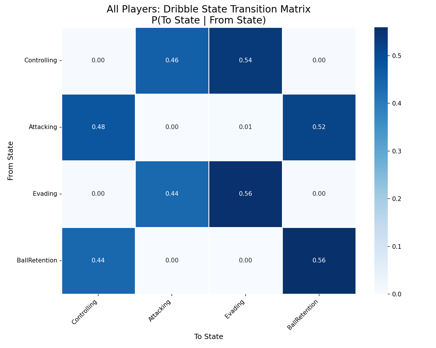
In the above matrix you see all hidden states as we calculated them for the Premier League 2025-2026 season. What you can see that there are values with 0,00 and that’s something that can be attributed to the small database in which we operate, but there are still a few interesting things happening here.
For example, if a player is in an attacking state – which we say a dribble is – we can see that the probability of the next tactical state is as follows:
- Keep in the attacking state → 0%
- Move towards a controling state → 48%
- Move towards an evading state → 0,01%
- Move towards a ball retention state → 52%
For me this doesn’t sit right, because it effectively says that after a dribble, the state is always a non-attacking one and always a form of control/ball retention. Let us give some more meaning to the locations of the dribbles begin and end + the areas of the pitch.
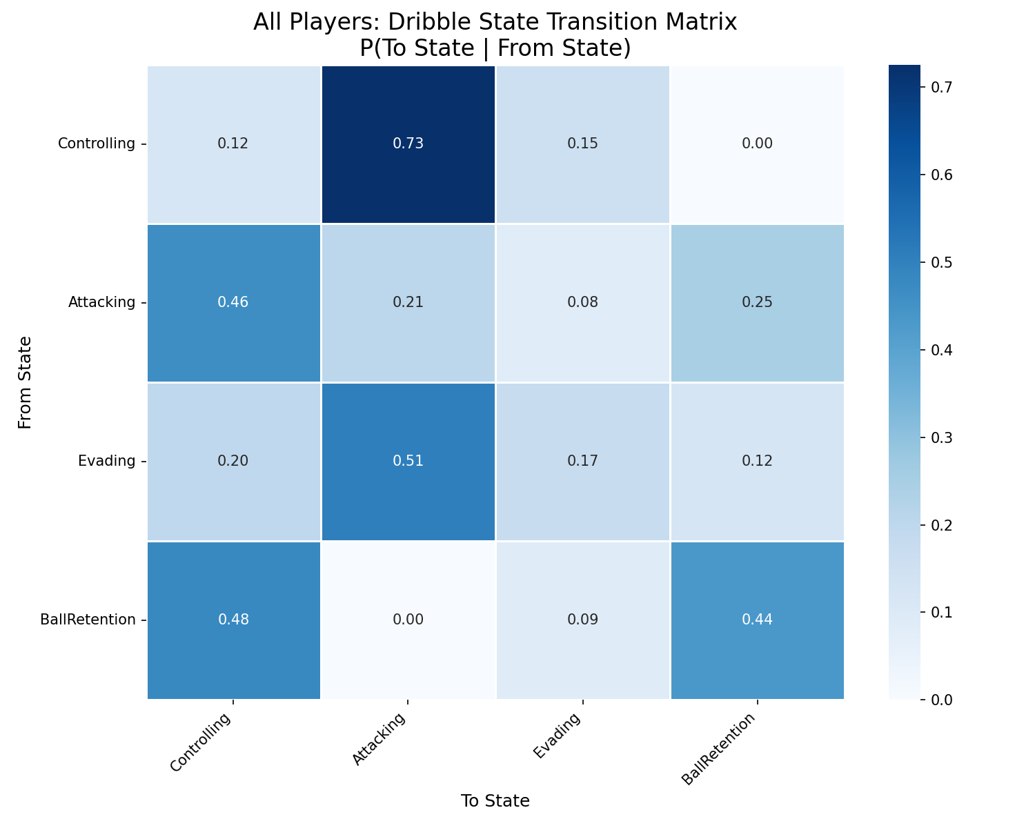
After making some alterations to the calculations, we see a very different matrix. In case of a dribble which is in an attacking state, how do the probabilities line up for the next action:
- Keep in the attacking state → 21%
- Move towards a controling state → 46%
- Move towards an evading state → 8%
- Move towards a ball retention state → 25%
That already looks like a more realistic scenario for dribbles. The most likely tactical state for a dribble to end in is a controling state followed by ball retention and attacking state. Dribbles in the Premier League are suggested to be very attacking and then resort to a more controlling state.
Now how does that look on a value grid for a pitch?
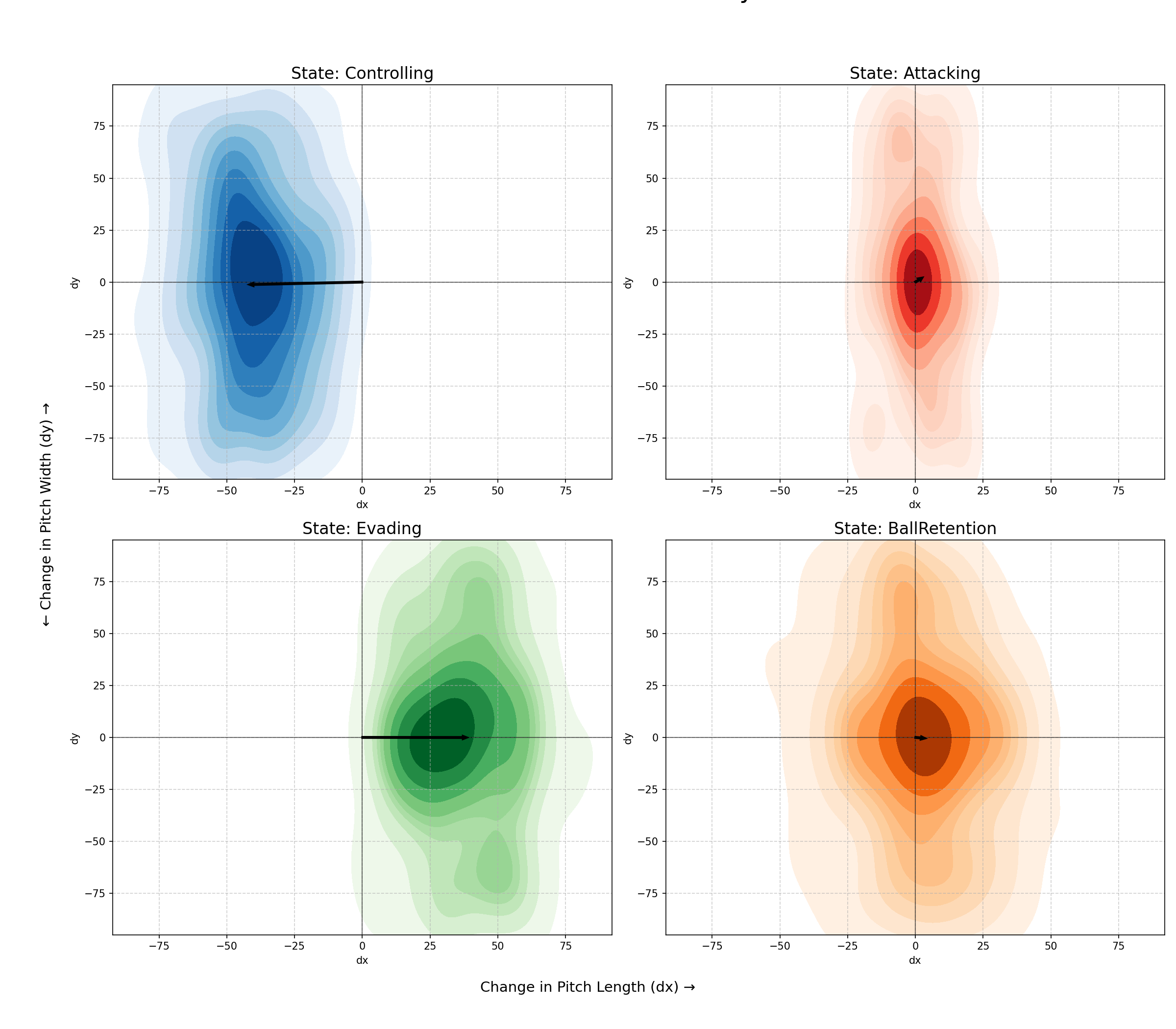
In the visual above you can see how the dribbles changed in their xy coordination. Controlliong and Evading change the most, while ball retention and the attacking state change the fewest. This means that the dribbles that stay in the attacking state have the shortest distance, while other more conservative states allow for more distance.
Let’s see how this looks for the players.
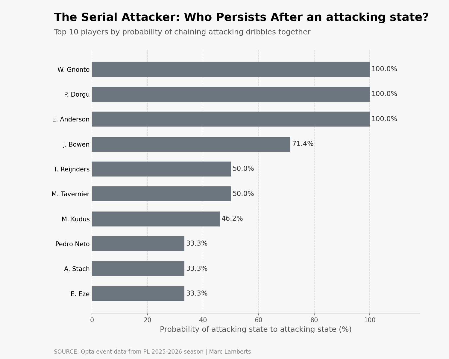
In the bar graph above you can see which players have dribbles where the next action also has the tactical state of attacking. In other words, they constantly look for an attacking option and pushing the ball forward.
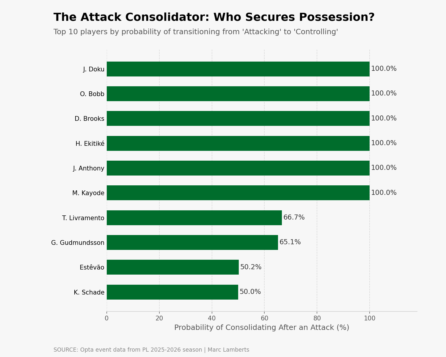
What I also think is interesting to see, is how players consolidate their dribbles after being in an attacking state: controlling state. Which players score highest in this? These players move towards more controlling areas or do make sure the ball ends up in a less threatening space but consolidates possession.
Challenges
The challenges are definitely present. First of all, I assign the states myself and I like to assign tactical states to data, which is quite sensitive to flaws. Why? Because I make a decision based on what I think is good, but also is very biased in a way. These are the challenges and critical things I need to think of, for next time:
- State definition: Tactical states are subjective and can introduce bias.
- Data limitations: Event data misses micro-actions; positional nuance is lost.
- Markov assumption: Transitions depend only on the previous state, ignoring broader context.
- Sparse events: Rare dribble outcomes can produce unstable probabilities.
- Interpretability: Statistical states may be hard to translate into footballing meaning.
- Player/context variability: Aggregated models may ignore individual style or team tactics.
- Scalability: Large datasets increase computational complexity.
- Validation: No ground truth for hidden tactical states; evaluation is subjective.
Final thoughts
Dribbles represent a complex and dynamic component of football, reflecting both individual skill and broader tactical intentions. The application of Hidden Markov Models provides a rigorous statistical framework to infer latent tactical states underlying observed actions, enabling an analytical perspective on progression, possession retention, and offensive transitions.
Despite inherent limitations — including subjective state definitions, data sparsity, and the absence of ground-truth labels for hidden states — this methodology demonstrates the potential of event-level analysis to bridge the gap between qualitative football insight and quantitative modeling. While the results should be interpreted cautiously, the approach underscores the value of combining domain knowledge with probabilistic modeling, contributing to a deeper understanding of player behavior, tactical dynamics, and the evaluative potential of high-resolution match data.
Sources
https://web.stanford.edu/~jurafsky/slp3/A.pdf
https://www.geeksforgeeks.org/machine-learning/hidden-markov-model-in-machine-learning/
Citation
admin. (2025, september 19). Using Hidden Markov Models on dribbles to see how much a dribble progresses attacks in the English Premier League 2025-2026.. Waltzing Analytics. https://waltzinganalytics.com/models/using-hidden-markov-models-on-dribbles-to-see-how-much-a-dribble-progresses-attacks-in-the-english-premier-league-2025-2026/