You can’t escape it if you are interested in football: Expected Goals (xG). Every football app has it listed with the shot data; you can’t open a social media app without seeing xG numbers or people speaking about it. In general, I think this is a positive development. I encourage speaking about data, but it does come with its pitfalls when we address more complicated and complex data models. And xG is one of them.
In this article, I want to have a look at what xG tells us about profiling and how different variables can have different outcomes. This is not an xG explainer, but a look at how we can take meaningful analysis from it towards the profiling of strikers. In other words, what can we conclude from xG that helps in scouting strikers?
The core of this article is entropy-adjusted xG: finding the share of the total xG that can be repeated under any circumstance, regardless of variables.
Data
The data I’m using for this is raw event data from Wyscout. This data was collected on February 8th, 2026. I’m well aware that the data points have changed for the ongoing season, but for our research, we have enough information to look ahead. The raw data is positional XY-data, and this specific data only focuses on on-ball actions. This means that we are depending on how xG is calculated by Wyscout and don’t look at what the players do for the entropy, that are not the shooter. The data I have collected focuses on five seasons of Premier League data, including the current ongoing 2025–2026 season.
The data comes in JSON-files, which is one my favourite types to handle data, and I have to flatten all the files before I can go to work. Expected goals are included as a separate column in the data, so we don’t have to create our own. We do, however, need to be critical of how Wyscout’s xG is calculated.
Because this analysis relies on Wyscout’s event tagging and expected-goals model, the results inherit the assumptions embedded in that system. Differences in how providers classify shot types, define pitch zones, or calibrate xG values may lead to slightly different entropy and stability scores.
The approach itself is provider-agnostic in principle, but the current implementation should be interpreted within the context of the underlying data model.
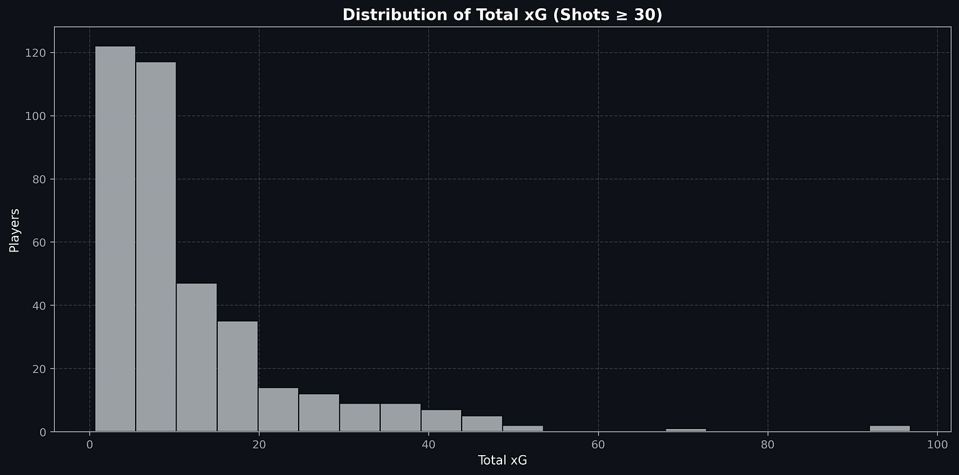
Entropy-based measures are sensitive to sample size. Players with fewer shots may appear artificially concentrated simply because their opportunity set is small, while very high-volume shooters will naturally show broader distributions.
To reduce this effect, the analysis applies minimum shot thresholds and uses aggregated multi-season data where possible. Comparisons are therefore most meaningful among players with similar shot volumes.
Stability should be interpreted as a profiling indicator rather than a precise individual parameter, especially for players near the inclusion threshold. Future extensions could incorporate smoothing or shrinkage techniques to stabilise low-sample estimates further.
Shot Stability
Shot stability is a simple way of describing how repeatable a player’s chances are. Two forwards can finish a season with the same expected goals total, but arrive there through very different shot profiles. One might rely on a steady stream of close-range chances from central areas, while another mixes those with speculative efforts from distance or low-probability angles. The first profile tends to be easier to reproduce over time; the second is often more dependent on game state, moments of space, or individual decisions. Stability, in this sense, is not about how good the shots are, but how consistently they come from the same kinds of situations.
To capture that idea, shot stability looks at how concentrated a player’s attempts are — in their location, their type, and their underlying chance value — and how often they occur in high-probability zones like the penalty area. Players whose shots cluster in similar areas and share similar characteristics score highly because their opportunities follow a clear, repeatable pattern. Players with a wider spread of locations and shot qualities score lower, reflecting a more volatile profile. By combining this information with traditional xG totals, we can separate chance volume from chance reliability and get a clearer picture of which scoring outputs are built on sustainable foundations.
Modelling Post-Save Rebound Sequences with Hidden Markov Models
Goalkeeper data analysis is one of the hardest things I have experienced doing in this space. So why do I keep…
Methodology
To move beyond raw xG totals, this analysis looks at how players generate their chances, not just how many they take. Using Wyscout event data, every non-penalty shot in the Premier League dataset is collected with its expected-goal value, location (XY), and shot details, then grouped by player. Instead of treating these shots as a simple count, each player’s attempts are viewed as a distribution of xG: some players build their numbers through a steady flow of similar chances, while others rely on a more unpredictable mix. The idea is to measure how concentrated or scattered that profile is and use that to estimate how repeatable their scoring opportunities really look.
To do that, the model calculates three measures of dispersion. The first looks at how evenly a player’s xG is spread across individual shots, whether it comes from lots of similar chances or a few big moments mixed with low-probability attempts. The second looks at where those shots come from, dividing the pitch into zones and measuring how tightly a player’s chances cluster in space. The third checks how varied the attempts are by shot type. These are paired with simple football indicators, such as how often a player shoots from inside the box or from central areas and how close to the goal their attempts tend to be. Together, these describe whether a player’s output comes from a clear, repeatable pattern or from a wider, more volatile spread of situations.
These elements are combined into a single stability score, kept on a simple 0–1 scale. Higher scores mean a player’s chances tend to come from consistent locations and situations; lower scores indicate a more scattered profile. That score is then used to weight each player’s total expected goals, producing an adjusted figure that reflects the share of their xG built on stable foundations. The result doesn’t replace traditional xG but adds another layer: separating the players who accumulate chances in a repeatable way from those whose totals depend more heavily on context, game flow, or one-off moments.
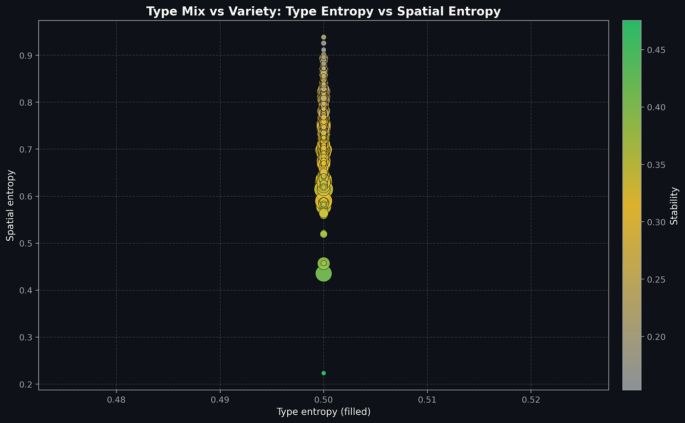
Shot Entropy
The first component of the model is shot entropy. Here, entropy is used as a measure of how evenly a player’s total xG is distributed across their individual attempts.
If a striker’s xG comes from many similar chances — for example, repeated shots worth around 0.15–0.20 xG — their distribution is concentrated and predictable. In entropy terms, this produces a lower entropy value, indicating a stable chance profile.
By contrast, a player who mixes a few very high-value chances with many speculative efforts has a more uneven distribution. Their total xG may look healthy, but it depends on a wider spread of shot qualities. This produces higher entropy, reflecting a more volatile profile.
Shot entropy, therefore, answers a simple question:
Is this player’s xG built from repeatable patterns, or from a mixture of very different situations?
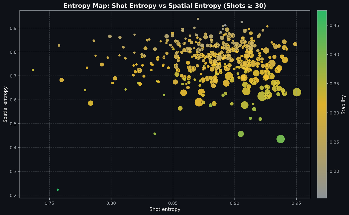
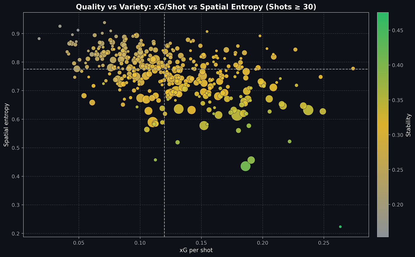
Spatial Entropy
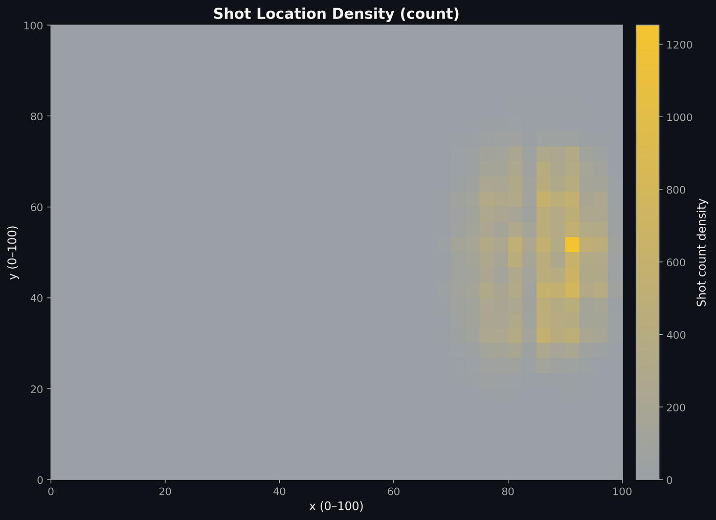
The second component is spatial entropy, which looks at where shots are taken from.
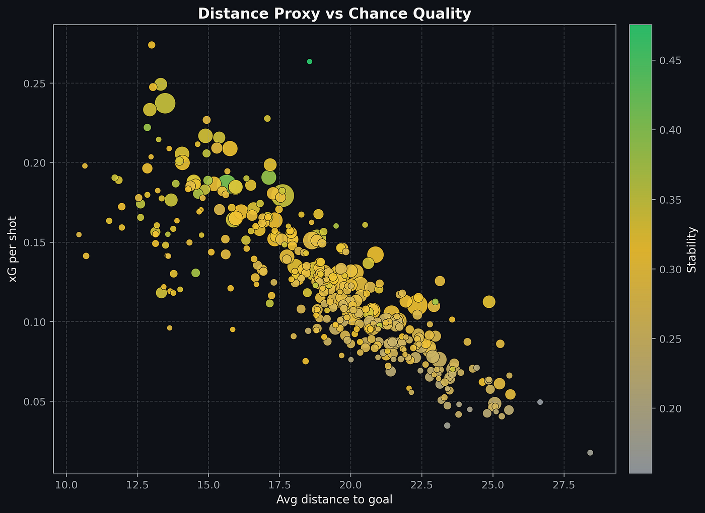
To measure this, the pitch is divided into zones, and each player’s xG is allocated across those zones. A player whose chances cluster in a few consistent areas, for example, central penalty-box positions, will show low spatial entropy. This indicates a clear and repeatable shot map.
Players who shoot from a wide variety of areas — outside the box, wide channels, deeper zones, or unusual angles — will show higher spatial entropy, reflecting a broader and less predictable spatial profile.
Importantly, this isn’t about whether the shots are good or bad. It’s about the consistency of location. A player who reliably arrives in the same dangerous spaces is generally easier to project forward than one whose shot locations depend heavily on match context or individual improvisation.
Shot Type Entropy
The third dispersion measure is shot type entropy, capturing how the attempts are taken.
This looks at the mix of shot categories recorded in the event data, for instance, headers, open-play shots, volleys, or other classifications provided by Wyscout. Players whose attempts mostly come from one or two consistent shot types will have lower entropy, suggesting their chances arise from a recognisable tactical pattern.
A striker heavily involved in crosses, for example, might show a strong concentration of headers and close-range finishes. Another forward who alternates between long-range strikes, rebounds, tight-angle shots, and occasional aerial chances will show a more varied profile and therefore higher entropy.
Shot type entropy helps distinguish between players whose finishing opportunities come from structured attacking patterns and those whose chances are more opportunistic.
Stability Formula
These three entropy measures — shot, spatial, and shot-type — are combined with simple football context indicators such as penalty-box shot share.
Rather than scaling or transforming the values into arbitrary scores, the model keeps everything interpretable on a 0–1 scale. Stability is calculated as a weighted combination of:
- lower shot entropy (more consistent chance quality)
- lower spatial entropy (more consistent shot locations)
- lower shot-type entropy (more consistent chance mechanics)
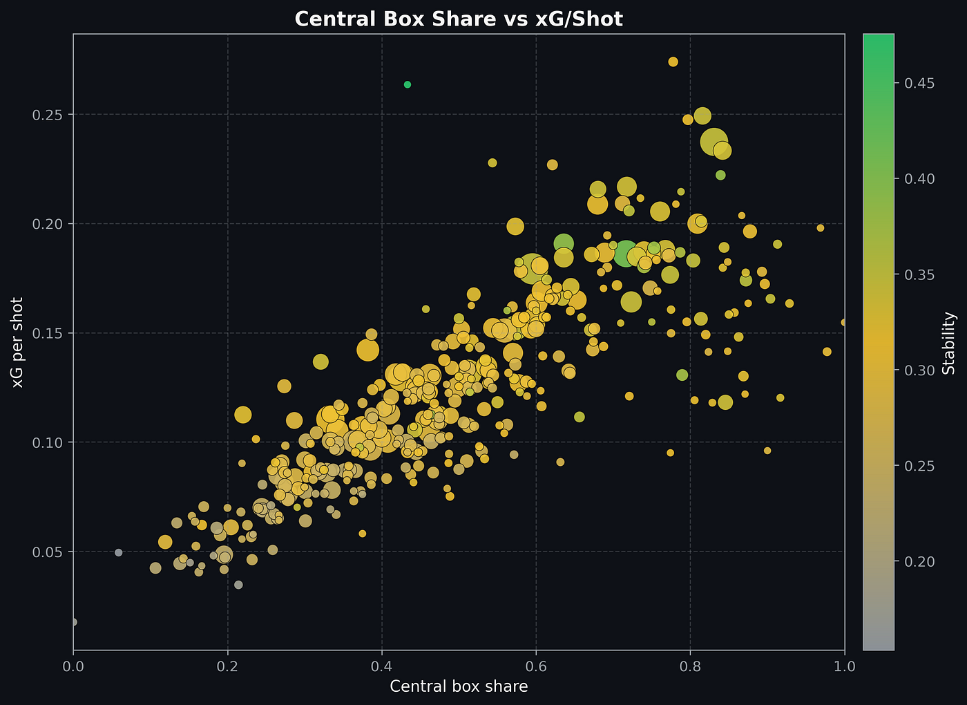
- higher share of shots from the penalty area
Conceptually, the formula rewards concentration and repeatability.
A player who repeatedly gets similar chances in similar places scores close to 1. A player whose chances come from many different situations scores closer to 0.
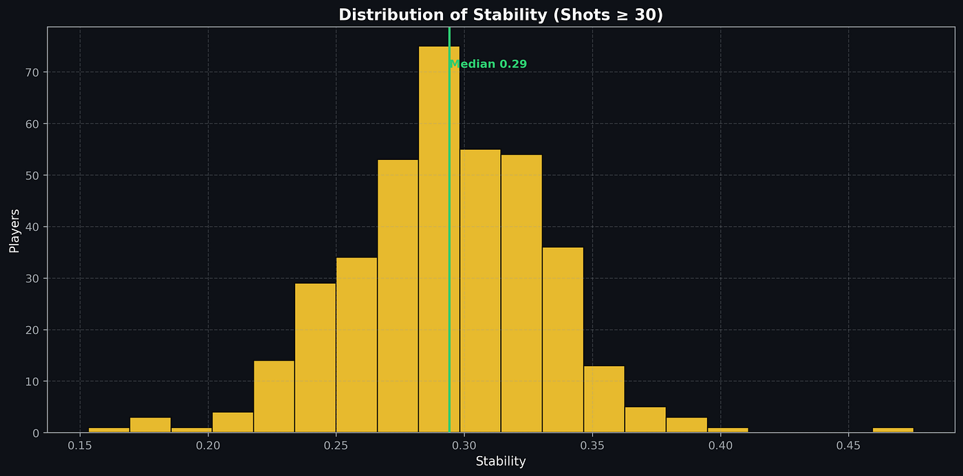
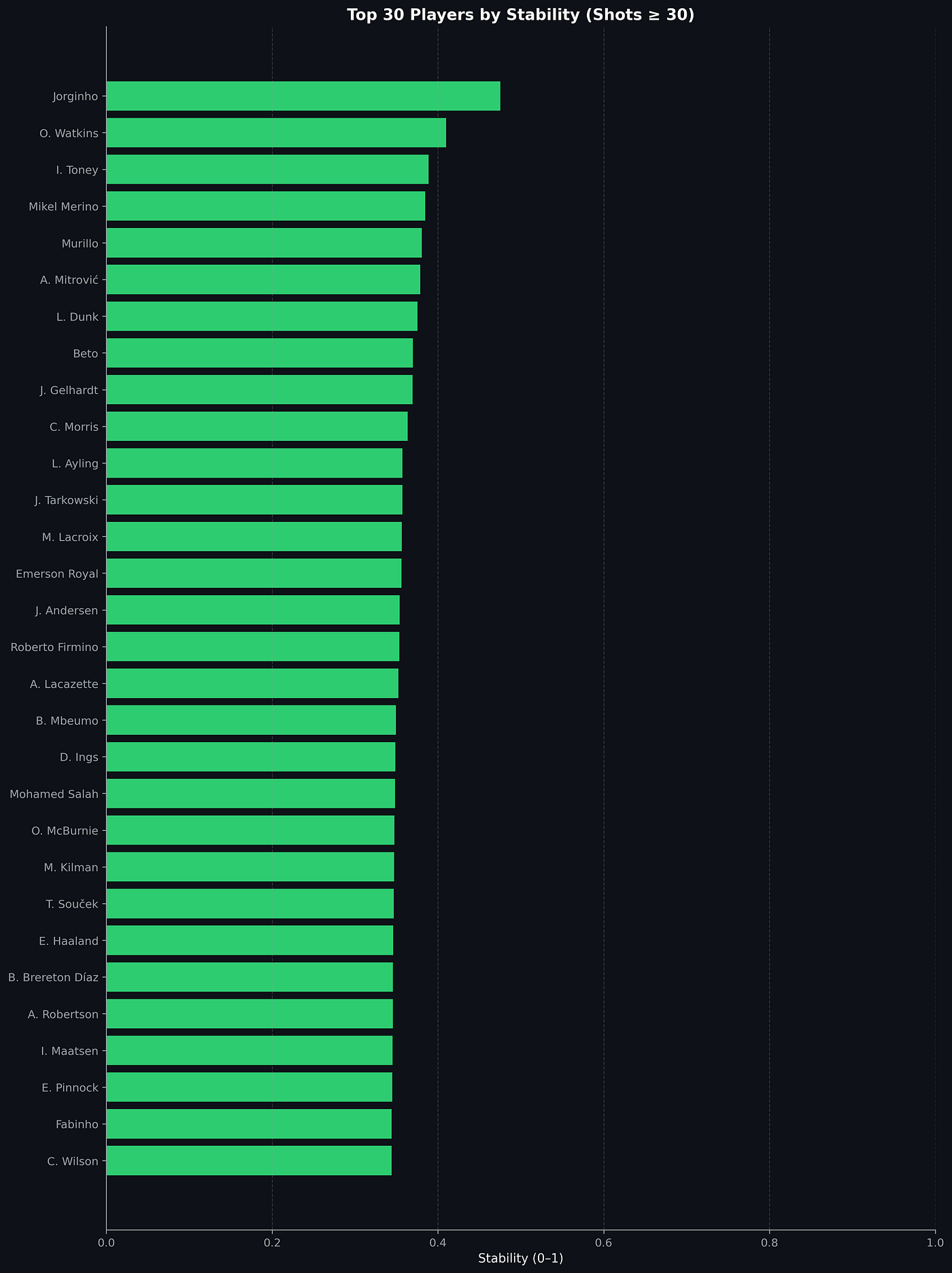
This produces a stability score that can be read intuitively:
- 0.80–1.00 → highly repeatable shot profile
- 0.60–0.79 → mostly structured but with some variation
- 0.40–0.59 → mixed profile
- below 0.40 → volatile or context-dependent shot generation
The exact number matters less than the interpretation: it reflects how much of a player’s attacking output appears structurally reliable.
Formal Stability Definition
To keep the model interpretable while still reproducible, stability is calculated as a weighted combination of normalized dispersion measures and contextual shot indicators.
Each entropy component is first scaled onto a 0–1 range:
- Shot entropy (Hq): dispersion of xG across attempts
- Spatial entropy (Hs): dispersion of xG across pitch zones
- Shot-type entropy (Ht): dispersion across shot categories
These are inverted so that higher values represent greater concentration:
Cq = 1 − Hq
Cs = 1 − Hs
Ct = 1 − Ht
A contextual indicator is then added:
Pb = share of shots taken inside the penalty area
Stability is defined as:
Stability = w1·Cq + w2·Cs + w3·Ct + w4·Pb
where the weights sum to 1.
For this study, equal weights are used for simplicity and interpretability, although alternative weightings could be explored depending on analytical priorities. This formulation keeps the score bounded between 0 and 1 while ensuring that higher values consistently reflect more repeatable shot profiles.
Adjusted xG
Once stability is calculated, it is applied directly to each player’s total expected goals:
xG-adj=xG x stability
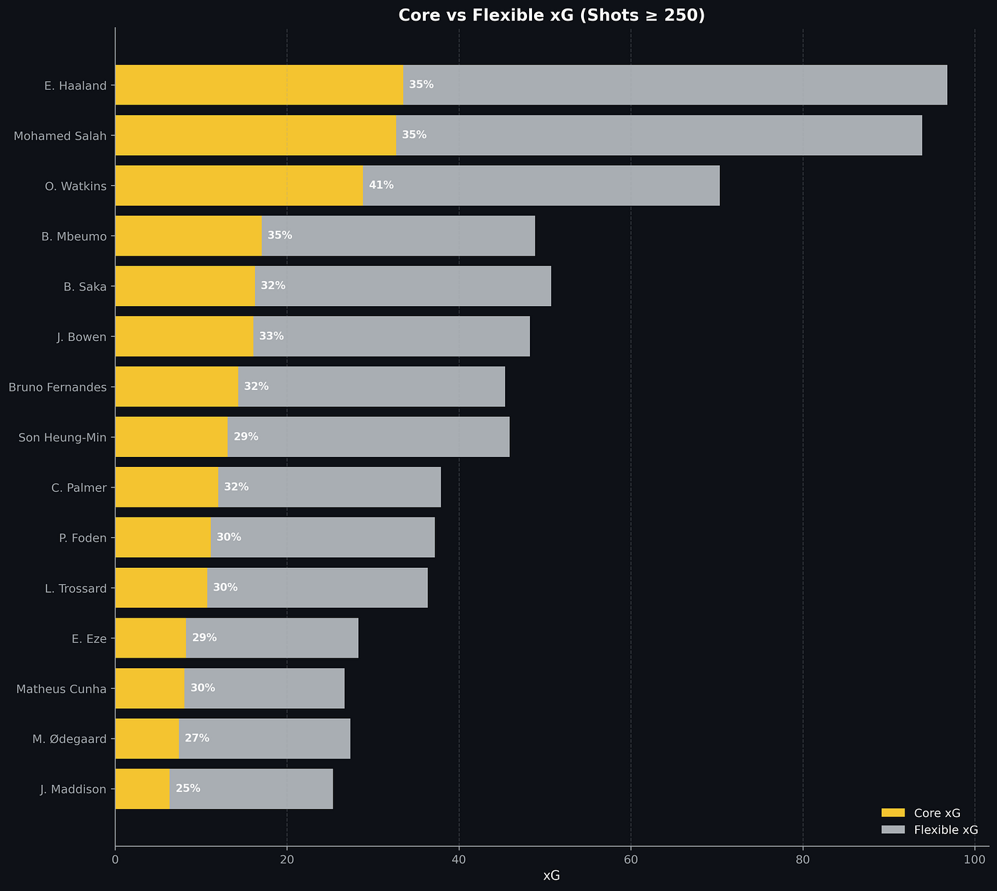
This produces entropy-adjusted expected goals (xG-adj), the portion of a player’s xG that comes from stable, repeatable shot patterns.
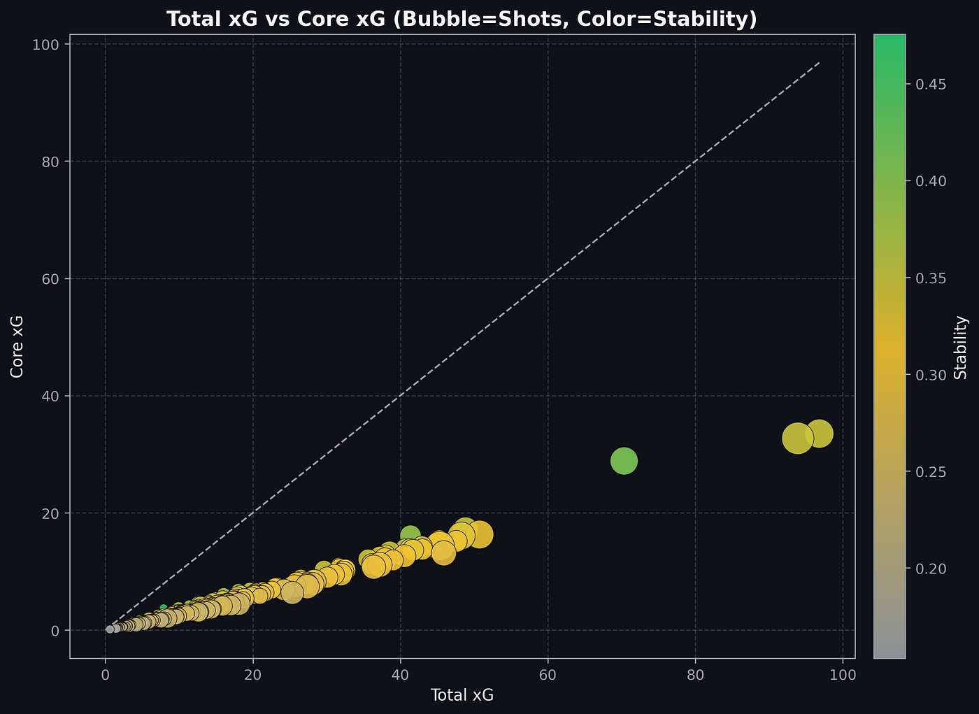
Because the stability score stays on a 0–1 scale, the interpretation remains simple:
- xG-adj = stable core of scoring opportunities
- xG − xG-adj = flexible or context-dependent opportunities
This does not mean the remaining xG is meaningless or “bad.”
Instead, it represents chances that may depend more on:
- specific tactical setups
- transition-heavy matches
- individual creativity
- unusual game states
The goal is not to penalise these players, but to separate sustainable volume from situational volume.
Two strikers can finish with 15 xG:
- Player A: 15 xG, stability 0.80 → 12.0 xG-adj
- Player B: 15 xG, stability 0.45 → 6.8 xG-adj
Both produced the same raw output, but the underlying shot profiles tell very different scouting stories.
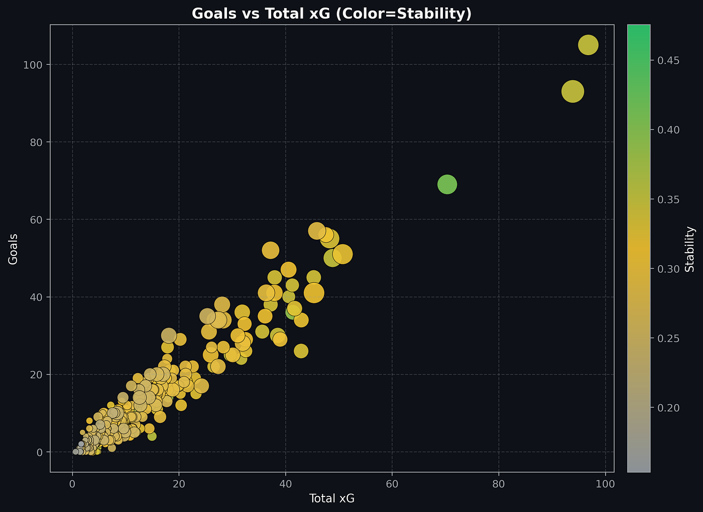
Results
Shot stability reflects not only a player’s tendencies, but also the attacking structure around them.
A striker in a highly structured possession system may consistently receive central penalty-area chances, producing a concentrated and repeatable shot profile. A forward in a fluid or transition-heavy side may generate attempts from a wider variety of positions and situations, resulting in higher entropy even if their individual quality is similar.
For this reason, stability should not be interpreted as a pure measure of player ability. Instead, it captures how a player’s opportunities emerge within a tactical context. When used in scouting, the metric is most informative when paired with an understanding of team style and expected role in a new system.
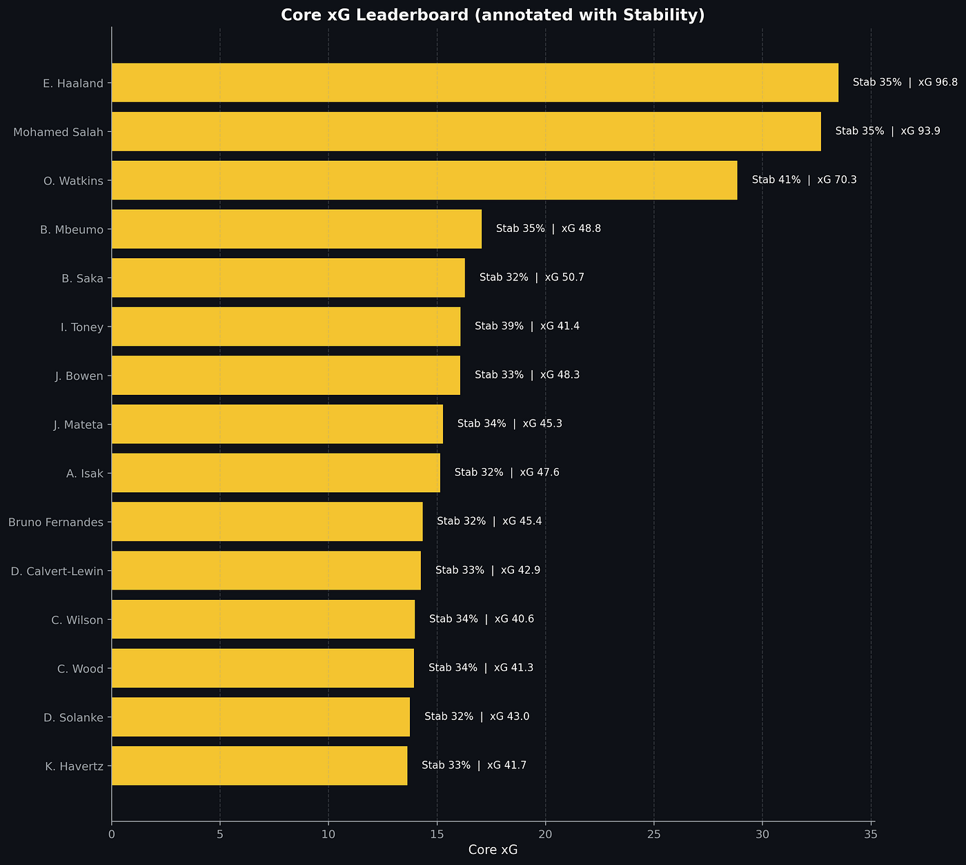
Applying this method to five Premier League seasons highlights clear stylistic differences between forwards.
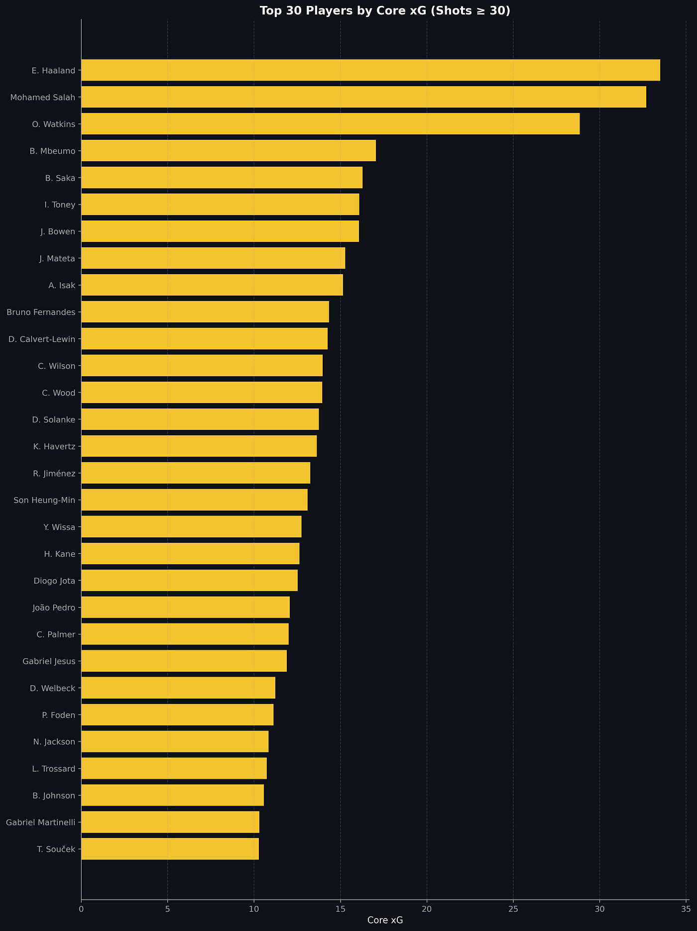
Some players maintain strong adjusted totals because their shot maps remain tightly focused in central box areas with consistent chance types. These players tend to profile as classic penalty-area strikers or system-driven finishers, whose opportunities arise from repeatable attacking patterns.
Others see their totals drop more noticeably after adjustment. These players may still be excellent attackers, but their shot generation relies more heavily on:
- long-range shooting
- varied positions across the front line
- transitional chaos rather than structured build-up
From a recruitment perspective, this distinction can be valuable. Clubs looking for a striker to plug into a structured possession system may prioritise players with higher stability. Teams relying on fluid attacking play or counter-attacks may be less concerned by lower stability scores.
The adjusted metric therefore, doesn’t rank players purely by output, but by the nature of that output.
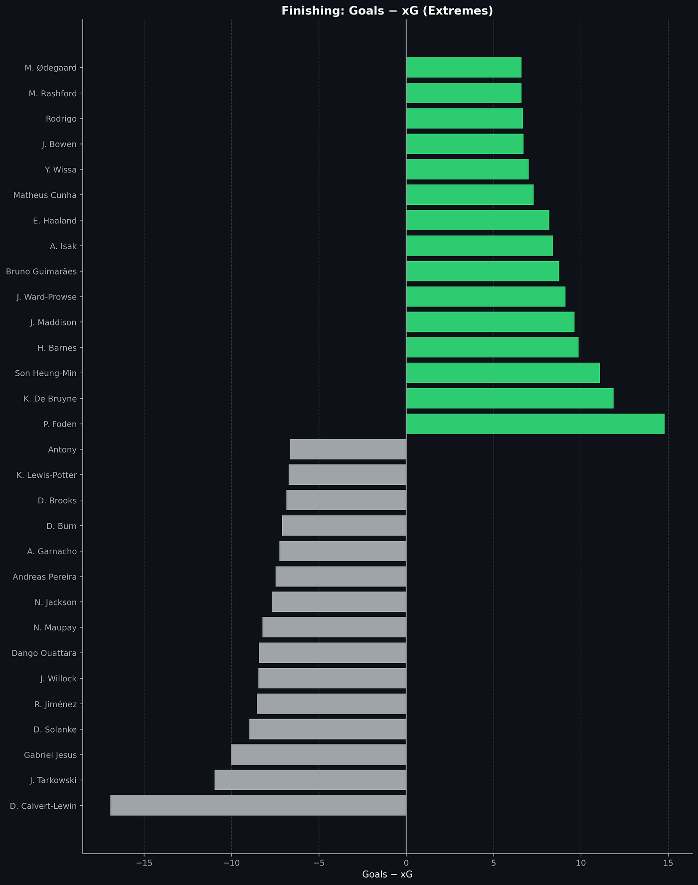
Final thoughts
Expected goals have transformed how we talk about finishing and attacking performance. But raw xG totals alone can blur important differences in how those chances are created.
Entropy-adjusted xG is an attempt to add one extra layer of interpretation. By measuring how concentrated a player’s shot profile is — in quality, location, and type — we can estimate how much of their scoring output comes from repeatable patterns versus more situational moments.
This doesn’t replace traditional xG, and it shouldn’t be used in isolation. Football remains too complex for any single metric to capture everything that matters. But as a profiling tool, stability-weighted xG can help separate:
- volume scorers from structural scorers
- system finishers from opportunistic shooters
- repeatable production from context-dependent output
And for scouting departments trying to project future performance rather than describe past results, that distinction can be the difference between a good signing and a great one. Finishing is rather different in that regard.
One of the motivations behind entropy-adjusted xG is its potential usefulness for projection rather than description.
Future work could test whether players with higher stability:
- maintain more consistent xG production from season to season
- show smaller performance swings after transfers
- or are easier to integrate into structured attacking systems
If stability improves predictive accuracy, it strengthens its value as a recruitment tool. Even if predictive gains are modest, the metric still offers a useful descriptive layer by clarifying how scoring opportunities are generated rather than simply how many occur.
Appendix